
10.1: Overview of Spectroscopy
- Page ID
- 220742

The focus of this chapter is on the interaction of ultraviolet, visible, and infrared radiation with matter. Because these techniques use optical materials to disperse and focus the radiation, they often are identified as optical spectroscopies. For convenience we will use the simpler term spectroscopy in place of optical spectroscopy; however, you should understand we will consider only a limited piece of what is a much broader area of analytical techniques.
Despite the difference in instrumentation, all spectroscopic techniques share several common features. Before we consider individual examples in greater detail, let’s take a moment to consider some of these similarities. As you work through the chapter, this overview will help you focus on the similarities between different spectroscopic methods of analysis. You will find it easier to understand a new analytical method when you can see its relationship to other similar methods.
What is Electromagnetic Radiation?
Electromagnetic radiation—light—is a form of energy whose behavior is described by the properties of both waves and particles. Some properties of electromagnetic radiation, such as its refraction when it passes from one medium to another (Figure \(\PageIndex{1}\)), are explained best when we describe light as a wave. Other properties, such as absorption and emission, are better described by treating light as a particle. The exact nature of electromagnetic radiation remains unclear, as it has since the development of quantum mechanics in the first quarter of the 20th century [Home, D.; Gribbin, J. New Scientist 1991, 2 Nov. 30–33]. Nevertheless, this dual model of wave and particle behavior provide a useful description for electromagnetic radiation.

Wave Properties of Electromagnetic Radiation
Electromagnetic radiation consists of oscillating electric and magnetic fields that propagate through space along a linear path and with a constant velocity. In a vacuum, electromagnetic radiation travels at the speed of light, c, which is \(2.99792 \times 10^8\) m/s. When electromagnetic radiation moves through a medium other than a vacuum, its velocity, v, is less than the speed of light in a vacuum. The difference between v and c is sufficiently small (<0.1%) that the speed of light to three significant figures, \(3.00 \times 10^8\) m/s, is accurate enough for most purposes.
The oscillations in the electric field and the magnetic field are perpendicular to each other and to the direction of the wave’s propagation. Figure \(\PageIndex{2}\) shows an example of plane-polarized electromagnetic radiation, which consists of a single oscillating electric field and a single oscillating magnetic field.
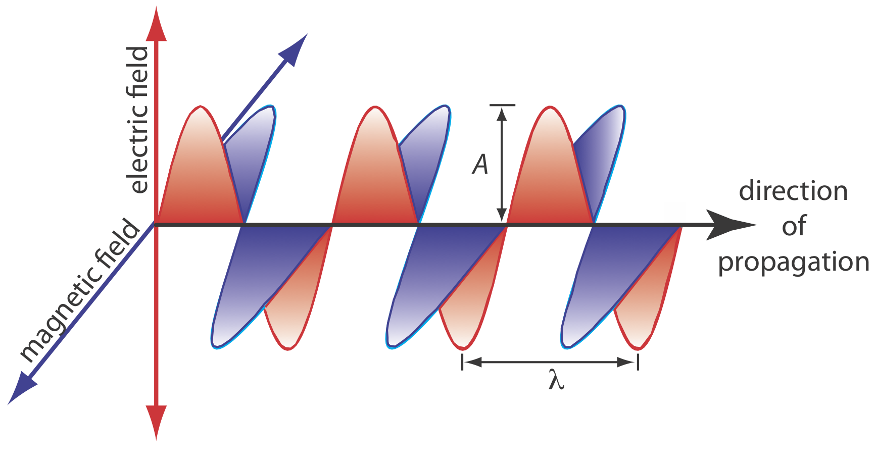
An electromagnetic wave is characterized by several fundamental properties, including its velocity, amplitude, frequency, phase angle, polarization, and direction of propagation [Ball, D. W. Spectroscopy 1994, 9(5), 24–25]. For example, the amplitude of the oscillating electric field at any point along the propagating wave is
\[A_{t}=A_{e} \sin (2 \pi \nu t+\Phi) \nonumber\]
where At is the magnitude of the electric field at time t, Ae is the electric field’s maximum amplitude, \(\nu\) is the wave’s frequency—the number of oscillations in the electric field per unit time—and \(\Phi\) is a phase angle that accounts for the fact that At need not have a value of zero at t = 0. The identical equation for the magnetic field is
\[A_{t}=A_{m} \sin (2 \pi \nu t+\Phi) \nonumber\]
where Am is the magnetic field’s maximum amplitude.
Other properties also are useful for characterizing the wave behavior of electromagnetic radiation. The wavelength, \(\lambda\), is defined as the distance between successive maxima (see Figure \(\PageIndex{2}\)). For ultraviolet and visible electromagnetic radiation the wavelength usually is expressed in nanometers (1 nm = 10–9 m), and for infrared radiation it is expressed in microns (1 mm = 10–6 m). The relationship between wavelength and frequency is
\[\lambda = \frac {c} {\nu} \nonumber\]
Another unit useful unit is the wavenumber, \(\overline{\nu}\), which is the reciprocal of wavelength
\[\overline{\nu} = \frac {1} {\lambda} \nonumber\]
Wavenumbers frequently are used to characterize infrared radiation, with the units given in cm–1.
When electromagnetic radiation moves between different media—for example, when it moves from air into water—its frequency, \(\nu\), remains constant. Because its velocity depends upon the medium in which it is traveling, the electromagnetic radiation’s wavelength, \(\lambda\), changes. If we replace the speed of light in a vacuum, c, with its speed in the medium, \(v\), then the wavelength is
\[\lambda = \frac {v} {\nu} \nonumber\]
This change in wavelength as light passes between two media explains the refraction of electromagnetic radiation shown in Figure \(\PageIndex{1}\).
In 1817, Josef Fraunhofer studied the spectrum of solar radiation, observing a continuous spectrum with numerous dark lines. Fraunhofer labeled the most prominent of the dark lines with letters. In 1859, Gustav Kirchhoff showed that the D line in the sun’s spectrum was due to the absorption of solar radiation by sodium atoms. The wavelength of the sodium D line is 589 nm. What are the frequency and the wavenumber for this line?
Solution
The frequency and wavenumber of the sodium D line are
\[\nu=\frac{c}{\lambda}=\frac{3.00 \times 10^{8} \ \mathrm{m} / \mathrm{s}}{589 \times 10^{-9} \ \mathrm{m}}=5.09 \times 10^{14} \ \mathrm{s}^{-1} \nonumber\]
\[\overline{\nu}=\frac{1}{\lambda}=\frac{1}{589 \times 10^{-9} \ \mathrm{m}} \times \frac{1 \ \mathrm{m}}{100 \ \mathrm{cm}}=1.70 \times 10^{4} \ \mathrm{cm}^{-1} \nonumber\]
Another historically important series of spectral lines is the Balmer series of emission lines from hydrogen. One of its lines has a wavelength of 656.3 nm. What are the frequency and the wavenumber for this line?
- Answer
-
The frequency and wavenumber for the line are
\[\nu=\frac{c}{\lambda}=\frac{3.00 \times 10^{8} \ \mathrm{m} / \mathrm{s}}{656.3 \times 10^{-9} \ \mathrm{m}}=4.57 \times 10^{14} \ \mathrm{s}^{-1} \nonumber\]
\[\overline{\nu}=\frac{1}{\lambda}=\frac{1}{656.3 \times 10^{-9} \ \mathrm{m}} \times \frac{1 \ \mathrm{m}}{100 \ \mathrm{cm}}=1.524 \times 10^{4} \ \mathrm{cm}^{-1} \nonumber\]
Particle Properties of Electromagnetic Radiation
When matter absorbs electromagnetic radiation it undergoes a change in energy. The interaction between matter and electromagnetic radiation is easiest to understand if we assume that radiation consists of a beam of energetic particles called photons. When a photon is absorbed by a sample it is “destroyed” and its energy acquired by the sample [Ball, D. W. Spectroscopy 1994, 9(6) 20–21]. The energy of a photon, in joules, is related to its frequency, wavelength, and wavenumber by the following equalities
\[E=h \nu=\frac{h c}{\lambda}=h c \overline{\nu} \nonumber\]
where h is Planck’s constant, which has a value of \(6.626 \times 10^{-34}\) Js.
What is the energy of a photon from the sodium D line at 589 nm?
Solution
The photon’s energy is
\[E=\frac{h c}{\lambda}=\frac{\left(6.626 \times 10^{-34} \ \mathrm{Js}\right)\left(3.00 \times 10^{8} \ \mathrm{m} / \mathrm{s}\right)}{589 \times 10^{-7} \ \mathrm{m}}=3.37 \times 10^{-19} \ \mathrm{J} \nonumber\]
What is the energy of a photon for the Balmer line at a wavelength of 656.3 nm?
- Answer
-
The photon’s energy is
\[E=\frac{h c}{\lambda}=\frac{\left(6.626 \times 10^{-34} \ \mathrm{Js}\right)\left(3.00 \times 10^{8} \ \mathrm{m} / \mathrm{s}\right)}{656.3 \times 10^{-9} \ \mathrm{m}}=3.03 \times 10^{-19} \ \mathrm{J} \nonumber\]
The Electromagnetic Spectrum
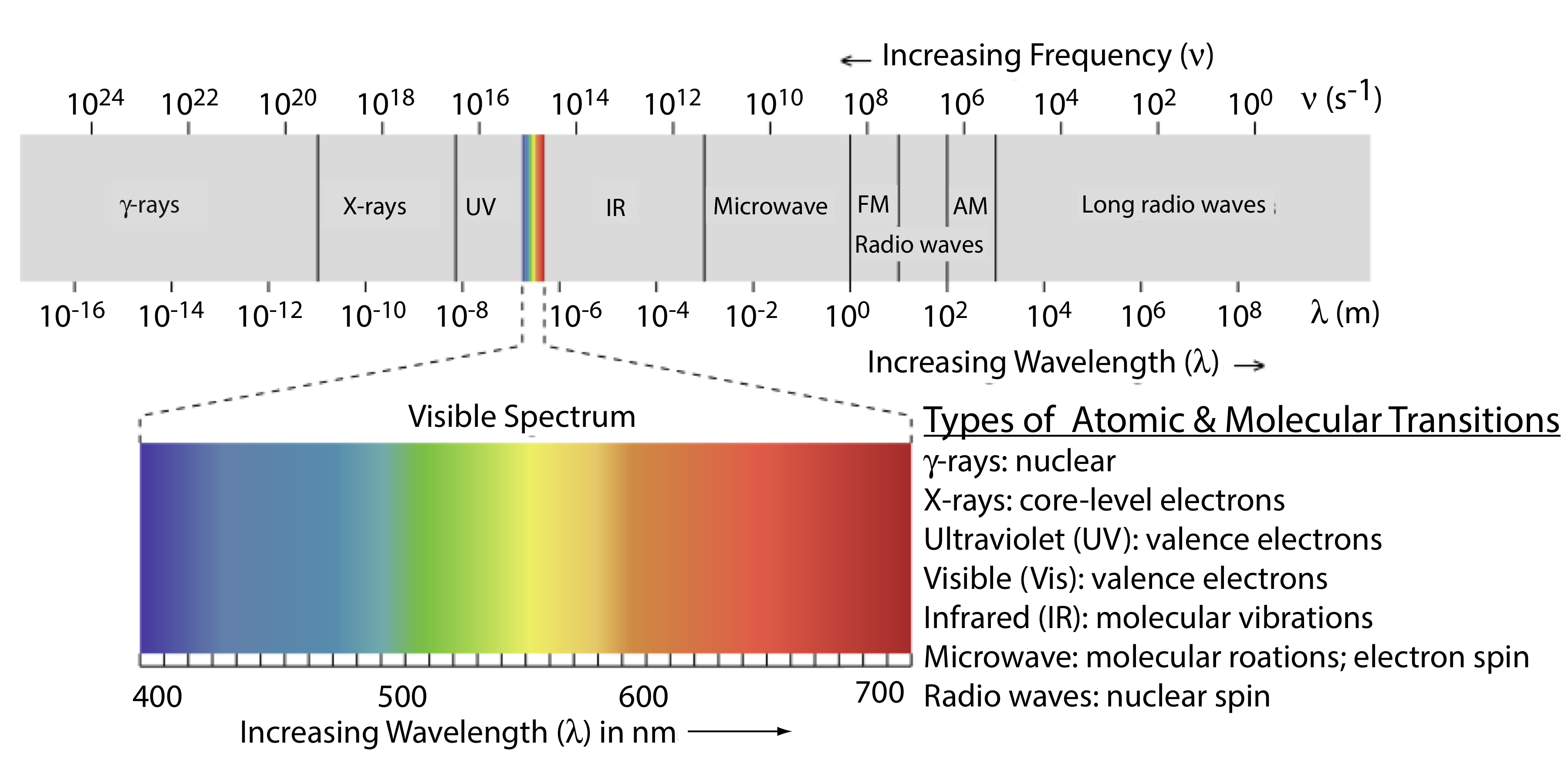
The frequency and the wavelength of electromagnetic radiation vary over many orders of magnitude. For convenience, we divide electromagnetic radiation into different regions—the electromagnetic spectrum—based on the type of atomic or molecular transitions that gives rise to the absorption or emission of photons (Figure \(\PageIndex{3}\)). The boundaries between the regions of the electromagnetic spectrum are not rigid and overlap between spectral regions is possible.
Photons as a Signal Source
In the previous section we defined several characteristic properties of electromagnetic radiation, including its energy, velocity, amplitude, frequency, phase angle, polarization, and direction of propagation. A spectroscopic measurement is possible only if the photon’s interaction with the sample leads to a change in one or more of these characteristic properties.
We will divide spectroscopy into two broad classes of techniques. In one class of techniques there is a transfer of energy between the photon and the sample. Table \(\PageIndex{1}\) provides a list of several representative examples.
In absorption spectroscopy a photon is absorbed by an atom or molecule, which undergoes a transition from a lower-energy state to a higher-energy, or excited state (Figure \(\PageIndex{4}\)). The type of transition depends on the photon’s energy. The electromagnetic spectrum in Figure \(\PageIndex{3}\), for example, shows that absorbing a photon of visible light promotes one of the atom’s or molecule’s valence electrons to a higher-energy level. When an molecule absorbs infrared radiation, on the other hand, one of its chemical bonds experiences a change in vibrational energy.
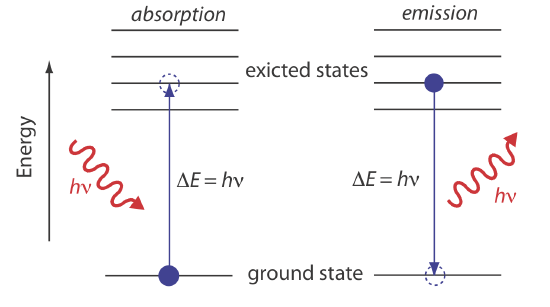
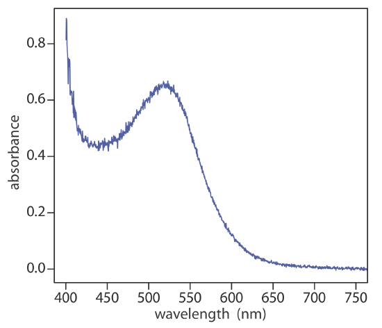
When it absorbs electromagnetic radiation the number of photons passing through a sample decreases. The measurement of this decrease in photons, which we call absorbance, is a useful analytical signal. Note that each energy level in Figure \(\PageIndex{4}\) has a well-defined value because each is quantized. Absorption occurs only when the photon’s energy, \(h \nu\), matches the difference in energy, \(\Delta E\), between two energy levels. A plot of absorbance as a function of the photon’s energy is called an absorbance spectrum. Figure \(\PageIndex{5}\), for example, shows the absorbance spectrum of cranberry juice.
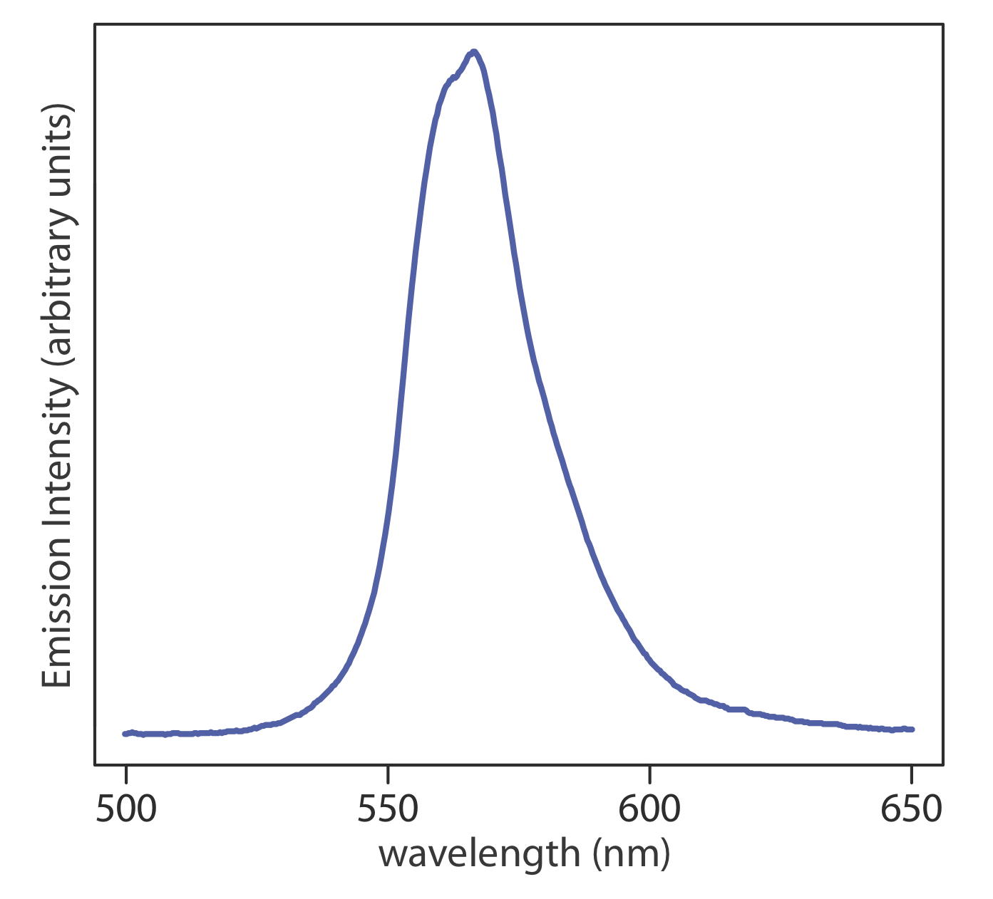
When an atom or molecule in an excited state returns to a lower energy state, the excess energy often is released as a photon, a process we call emission (Figure \(\PageIndex{4}\)). There are several ways in which an atom or a molecule may end up in an excited state, including thermal energy, absorption of a photon, or as the result of a chemical reaction. Emission following the absorption of a photon is also called photoluminescence, and that following a chemical reaction is called chemiluminescence. A typical emission spectrum is shown in Figure \(\PageIndex{6}\).
Molecules also can release energy in the form of heat. We will return to this point later in the chapter.

Figure \(\PageIndex{6}\). Photoluminescence spectrum of the dye coumarin 343, which is incorporated in a reverse micelle suspended in cyclohexanol. The dye’s absorbance spectrum (not shown) has a broad peak around 400 nm. The sharp peak at 409 nm is from the laser source used to excite coumarin 343. The broad band centered at approximately 500 nm is the dye’s emission band. Because the dye absorbs blue light, a solution of coumarin 343 appears yellow in the absence of photoluminescence. Its photoluminescent emission is blue-green. Source: data from Bridget Gourley, Department of Chemistry & Biochemistry, DePauw University.
In the second broad class of spectroscopic techniques, the electromagnetic radiation undergoes a change in amplitude, phase angle, polarization, or direction of propagation as a result of its refraction, reflection, scattering, diffraction, or dispersion by the sample. Several representative spectroscopic techniques are listed in Table \(\PageIndex{2}\).
Basic Components of Spectroscopic Instruments
The spectroscopic techniques in Table \(\PageIndex{1}\) and Table \(\PageIndex{2}\) use instruments that share several common basic components, including a source of energy, a means for isolating a narrow range of wavelengths, a detector for measuring the signal, and a signal processor that displays the signal in a form convenient for the analyst. In this section we introduce these basic components. Specific instrument designs are considered in later sections.
You will find a more detailed treatment of these components in the additional resources for this chapter.
Sources of Energy
All forms of spectroscopy require a source of energy. In absorption and scattering spectroscopy this energy is supplied by photons. Emission and photoluminescence spectroscopy use thermal, radiant (photon), or chemical energy to promote the analyte to a suitable excited state.
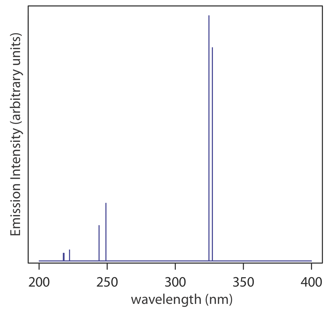
Sources of Electromagnetic Radiation. A source of electromagnetic radiation must provide an output that is both intense and stable. Sources of electromagnetic radiation are classified as either continuum or line sources. A continuum source emits radiation over a broad range of wavelengths, with a relatively smooth variation in intensity (Figure \(\PageIndex{7}\)). A line source, on the other hand, emits radiation at selected wavelengths (Figure \(\PageIndex{8}\)). Table \(\PageIndex{3}\) provides a list of the most common sources of electromagnetic radiation.
Sources of Thermal Radiation. The most common sources of thermal energy are flames and plasmas. A flame source uses a combustion of a fuel and an oxidant to achieve temperatures of 2000–3400 K. Plasmas, which are hot, ionized gases, provide temperatures of 6000–10000 K.
Chemical Sources of Energy. Exothermic reactions also may serve as a source of energy. In chemiluminescence the analyte is raised to a higher-energy state by means of a chemical reaction, emitting characteristic radiation when it returns to a lower-energy state. When the chemical reaction results from a biological or enzymatic reaction, the emission of radiation is called bioluminescence. Commercially available “light sticks” and the flash of light from a firefly are examples of chemiluminescence and bioluminescence.
Wavelength Selection
In Nessler’s original colorimetric method for ammonia, which was described at the beginning of the chapter, the sample and several standard solutions of ammonia are placed in separate tall, flat-bottomed tubes. As shown in Figure \(\PageIndex{9}\), after adding the reagents and allowing the color to develop, the analyst evaluates the color by passing ambient light through the bottom of the tubes and looking down through the solutions. By matching the sample’s color to that of a standard, the analyst is able to determine the concentration of ammonia in the sample.
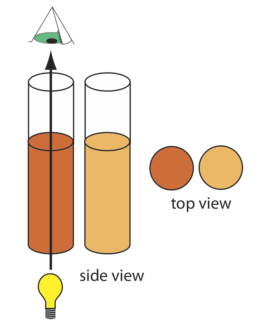
In Figure \(\PageIndex{9}\) every wavelength of light from the source passes through the sample. This is not a problem if there is only one absorbing species in the sample. If the sample contains two components, then a quantitative analysis using Nessler’s original method is impossible unless the standards contains the second component at the same concentration it has in the sample.
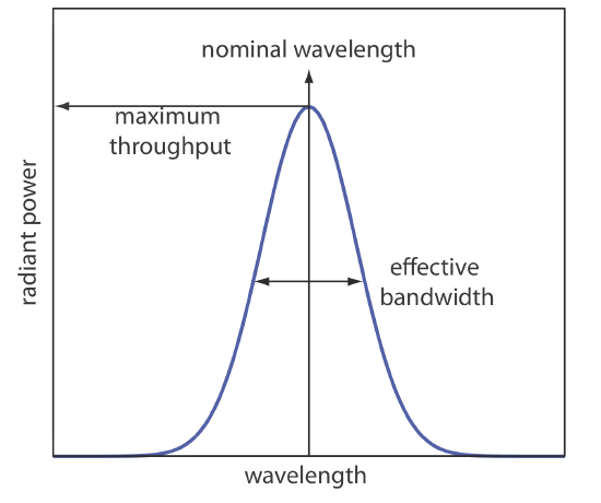
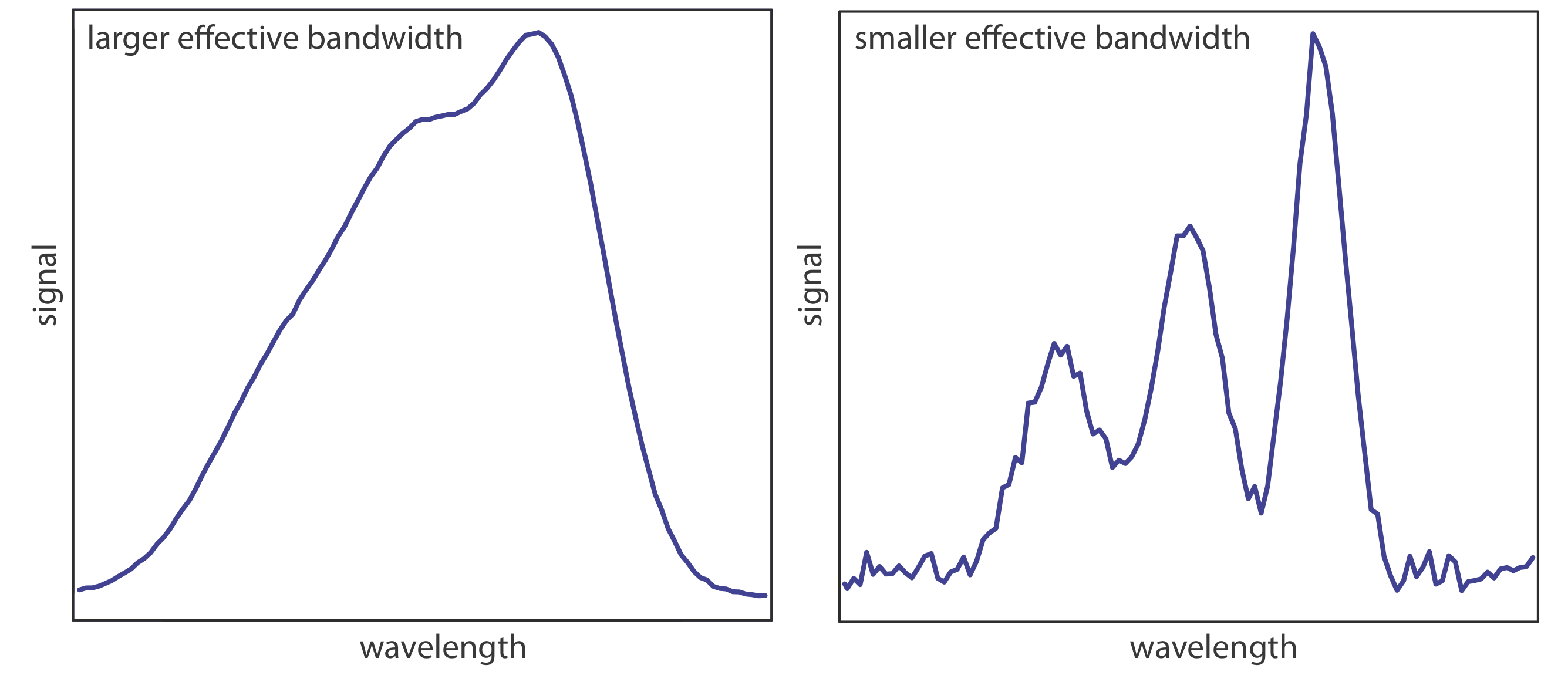
To overcome this problem, we want to select a wavelength that only the analyte absorbs. Unfortunately, we can not isolate a single wavelength of radiation from a continuum source, although we can narrow the range of wavelengths that reach the sample. As seen in Figure \(\PageIndex{10}\), a wavelength selector always passes a narrow band of radiation characterized by a nominal wavelength, an effective bandwidth, and a maximum throughput of radiation. The effective bandwidth is defined as the width of the radiation at half of its maximum throughput.
The ideal wavelength selector has a high throughput of radiation and a narrow effective bandwidth. A high throughput is desirable because the more photons that pass through the wavelength selector, the stronger the signal and the smaller the background noise. A narrow effective bandwidth provides a higher resolution, with spectral features separated by more than twice the effective bandwidth being resolved. As shown in Figure \(\PageIndex{11}\), these two features of a wavelength selector often are in opposition. A larger effective bandwidth favors a higher throughput of radiation, but provide less resolution. Decreasing the effective bandwidth improves resolution, but at the cost of a noisier signal [Jiang, S.; Parker, G. A. Am. Lab. 1981, October, 38–43]. For a qualitative analysis, resolution usually is more important than noise and a smaller effective bandwidth is desirable; however, in a quantitative analysis less noise usually is desirable.
Wavelength Selection Using Filters. The simplest method for isolating a narrow band of radiation is to use an absorption or interference filter. Absorption filters work by selectively absorbing radiation from a narrow region of the electromagnetic spectrum. Interference filters use constructive and destructive interference to isolate a narrow range of wavelengths. A simple example of an absorption filter is a piece of colored glass. A purple filter, for example, removes the complementary color green from 500–560 nm.
Commercially available absorption filters provide effective bandwidths of 30–250 nm, although the throughput at the low end of this range often is only 10% of the source’s emission intensity. Interference filters are more expensive than absorption filters, but have narrower effective bandwidths, typically 10–20 nm, with maximum throughputs of at least 40%.
Wavelength Selection Using Monochromators. A filter has one significant limitation—because a filter has a fixed nominal wavelength, if we need to make measurements at two different wavelengths, then we must use two different filters. A monochromator is an alternative method for selecting a narrow band of radiation that also allows us to continuously adjust the band’s nominal wavelength.
The construction of a typical monochromator is shown in Figure \(\PageIndex{12}\). Radiation from the source enters the monochromator through an entrance slit. The radiation is collected by a collimating mirror, which reflects a parallel beam of radiation to a diffraction grating. The diffraction grating is an optically reflecting surface with a large number of parallel grooves (see insert to Figure \(\PageIndex{12}\)). The diffraction grating disperses the radiation and a second mirror focuses the radiation onto a planar surface that contains an exit slit. In some monochromators a prism is used in place of the diffraction grating.
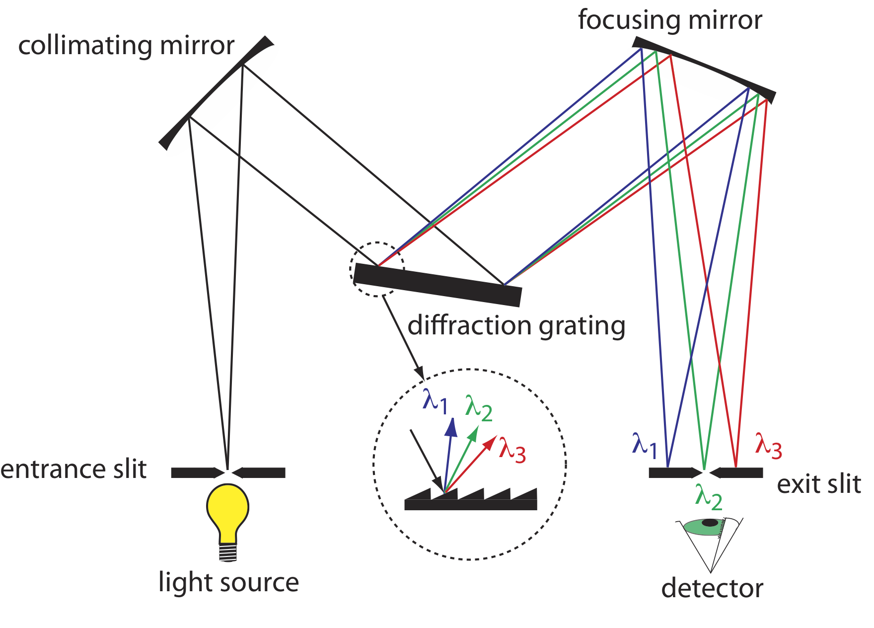
Radiation exits the monochromator and passes to the detector. As shown in Figure \(\PageIndex{12}\), a monochromator converts a polychromatic source of radiation at the entrance slit to a monochromatic source of finite effective bandwidth at the exit slit. The choice of which wavelength exits the monochromator is determined by rotating the diffraction grating. A narrower exit slit provides a smaller effective bandwidth and better resolution than does a wider exit slit, but at the cost of a smaller throughput of radiation.
Polychromatic means many colored. Polychromatic radiation contains many different wavelengths of light. Monochromatic means one color, or one wavelength. Although the light exiting a monochromator is not strictly of a single wavelength, its narrow effective bandwidth allows us to think of it as monochromatic.
Monochromators are classified as either fixed-wavelength or scanning. In a fixed-wavelength monochromator we manually select the wavelength by rotating the grating. Normally a fixed-wavelength monochromator is used for a quantitative analysis where measurements are made at one or two wavelengths. A scanning monochromator includes a drive mechanism that continuously rotates the grating, which allows successive wavelengths of light to exit from the monochromator. A scanning monochromator is used to acquire spectra, and, when operated in a fixed-wavelength mode, for a quantitative analysis.
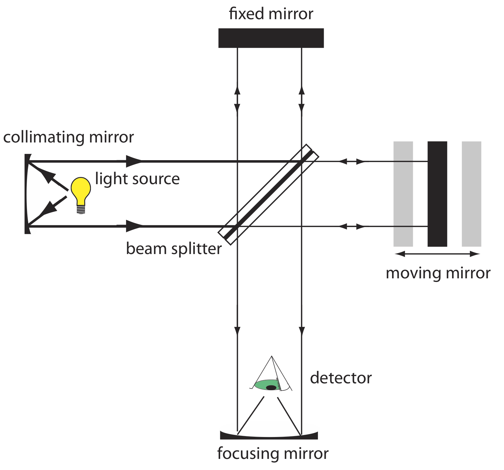
Interferometers. An interferometer provides an alternative approach for wavelength selection. Instead of filtering or dispersing the electromagnetic radiation, an interferometer allows source radiation of all wavelengths to reach the detector simultaneously (Figure \(\PageIndex{13}\)). Radiation from the source is focused on a beam splitter that reflects half of the radiation to a fixed mirror and transmits the other half to a moving mirror. The radiation recombines at the beam splitter, where constructive and destructive interference determines, for each wavelength, the intensity of light that reaches the detector. As the moving mirror changes position, the wavelength of light that experiences maximum constructive interference and maximum destructive interference also changes. The signal at the detector shows intensity as a function of the moving mirror’s position, expressed in units of distance or time. The result is called an interferogram or a time domain spectrum. The time domain spectrum is converted mathematically, by a process called a Fourier transform, to a spectrum (a frequency domain spectrum) that shows intensity as a function of the radiation’s energy.
The mathematical details of the Fourier transform are beyond the level of this textbook. You can consult the chapter’s additional resources for additional information.
In comparison to a monochromator, an interferometer has two significant advantages. The first advantage, which is termed Jacquinot’s advantage, is the greater throughput of source radiation. Because an interferometer does not use slits and has fewer optical components from which radiation is scattered and lost, the throughput of radiation reaching the detector is \(80-200 \times\) greater than that for a monochromator. The result is less noise. The second advantage, which is called Fellgett’s advantage, is a savings in the time needed to obtain a spectrum. Because the detector monitors all frequencies simultaneously, a spectrum takes approximately one second to record, as compared to 10–15 minutes when using a scanning monochromator.
Detectors
In Nessler’s original method for determining ammonia (Figure \(\PageIndex{9}\)) the analyst’s eye serves as the detector, matching the sample’s color to that of a standard. The human eye, of course, has a poor range—it responds only to visible light—and it is not particularly sensitive or accurate. Modern detectors use a sensitive transducer to convert a signal consisting of photons into an easily measured electrical signal. Ideally the detector’s signal, S, is a linear function of the electromagnetic radiation’s power, P,
\[S=k P+D \nonumber\]
where k is the detector’s sensitivity, and D is the detector’s dark current, or the background current when we prevent the source’s radiation from reaching the detector.
There are two broad classes of spectroscopic transducers: thermal transducers and photon transducers. Table \(\PageIndex{4}\) provides several representative examples of each class of transducers.
Transducer is a general term that refers to any device that converts a chemical or a physical property into an easily measured electrical signal. The retina in your eye, for example, is a transducer that converts photons into an electrical nerve impulse; your eardrum is a transducer that converts sound waves into a different electrical nerve impulse.
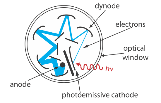
Photon Transducers. Phototubes and photomultipliers use a photosensitive surface that absorbs radiation in the ultraviolet, visible, or near IR to produce an electrical current that is proportional to the number of photons reaching the transducer (Figure \(\PageIndex{14}\)). Other photon detectors use a semiconductor as the photosensitive surface. When the semiconductor absorbs photons, valence electrons move to the semiconductor’s conduction band, producing a measurable current. One advantage of the Si photodiode is that it is easy to miniaturize. Groups of photodiodes are gathered together in a linear array that contains 64–4096 individual photodiodes. With a width of 25 μm per diode, a linear array of 2048 photodiodes requires only 51.2 mm of linear space. By placing a photodiode array along the monochromator’s focal plane, it is possible to monitor simultaneously an entire range of wavelengths.
Thermal Transducers. Infrared photons do not have enough energy to produce a measurable current with a photon transducer. A thermal transducer, therefore, is used for infrared spectroscopy. The absorption of infrared photons increases a thermal transducer’s temperature, changing one or more of its characteristic properties. A pneumatic transducer, for example, is a small tube of xenon gas with an IR transparent window at one end and a flexible membrane at the other end. Photons enter the tube and are absorbed by a blackened surface, increasing the temperature of the gas. As the temperature inside the tube fluctuates, the gas expands and contracts and the flexible membrane moves in and out. Monitoring the membrane’s displacement produces an electrical signal.
Signal Processors
A transducer’s electrical signal is sent to a signal processor where it is displayed in a form that is more convenient for the analyst. Examples of signal processors include analog or digital meters, recorders, and computers equipped with digital acquisition boards. A signal processor also is used to calibrate the detector’s response, to amplify the transducer’s signal, to remove noise by filtering, or to mathematically transform the signal.
If the retina in your eye and the eardrum in your ear are transducers, then your brain is the signal processor.