
9.2: Acid–Base Titrations
- Page ID
- 220734

Before 1800, most acid–base titrations used H2SO4, HCl, or HNO3 as acidic titrants, and K2CO3 or Na2CO3 as basic titrants. A titration’s end point was determined using litmus as an indicator, which is red in acidic solutions and blue in basic solutions, or by the cessation of CO2 effervescence when neutralizing \(\text{CO}_3^{2-}\) . Early examples of acid–base titrimetry include determining the acidity or alkalinity of solutions, and determining the purity of carbonates and alkaline earth oxides.
The determination of acidity and alkalinity continue to be important applications of acid–base titrimetry. We will take a closer look at these applications later in this section.
Three limitations slowed the development of acid–base titrimetry: the lack of a strong base titrant for the analysis of weak acids, the lack of suitable indicators, and the absence of a theory of acid–base reactivity. The introduction, in 1846, of NaOH as a strong base titrant extended acid–base titrimetry to the determination of weak acids. The synthesis of organic dyes provided many new indicators. Phenolphthalein, for example, was first synthesized by Bayer in 1871 and used as an indicator for acid–base titrations in 1877.
Despite the increased availability of indicators, the absence of a theory of acid–base reactivity made it difficult to select an indicator. The development of equilibrium theory in the late 19th century led to significant improvements in the theoretical understanding of acid–base chemistry, and, in turn, of acid–base titrimetry. Sørenson’s establishment of the pH scale in 1909 provided a rigorous means to compare indicators. The determination of acid–base dissociation constants made it possible to calculate a theoretical titration curve, as outlined by Bjerrum in 1914. For the first time analytical chemists had a rational method for selecting an indicator, making acid–base titrimetry a useful alternative to gravimetry.
Acid–Base Titration Curves
In the overview to this chapter we noted that a titration’s end point should coincide with its equivalence point. To understand the relationship between an acid–base titration’s end point and its equivalence point we must know how the titrand’s pH changes during a titration. In this section we will learn how to calculate a titration curve using the equilibrium calculations from Chapter 6. We also will learn how to sketch a good approximation of any acid–base titration curve using a limited number of simple calculations.
Titrating Strong Acids and Strong Bases
For our first titration curve, let’s consider the titration of 50.0 mL of 0.100 M HCl using a titrant of 0.200 M NaOH. When a strong base and a strong acid react the only reaction of importance is
\[\mathrm{H}_{3} \mathrm{O}^{+}(a q)+\mathrm{OH}^{-}(a q) \rightarrow 2 \mathrm{H}_{2} \mathrm{O}(\mathrm{l}) \label{9.1}\]
Although we have not written reaction \ref{9.1} as an equilibrium reaction, it is at equilibrium; however, because its equilibrium constant is large—it is (Kw)–1 or \(1.00 \times 10^{14}\)—we can treat reaction \ref{9.1} as though it goes to completion.
The first task is to calculate the volume of NaOH needed to reach the equivalence point, Veq. At the equivalence point we know from reaction \ref{9.1} that
\[\begin{aligned} \text { moles } \mathrm{HCl}=& \text { moles } \mathrm{NaOH} \\ M_{a} \times V_{a} &=M_{b} \times V_{b} \end{aligned} \nonumber\]
where the subscript ‘a’ indicates the acid, HCl, and the subscript ‘b’ indicates the base, NaOH. The volume of NaOH needed to reach the equivalence point is
\[V_{e q}=V_{b}=\frac{M_{a} V_{a}}{M_{b}}=\frac{(0.100 \ \mathrm{M})(50.0 \ \mathrm{mL})}{(0.200 \ \mathrm{M})}=25.0 \ \mathrm{mL} \nonumber\]
Before the equivalence point, HCl is present in excess and the pH is determined by the concentration of unreacted HCl. At the start of the titration the solution is 0.100 M in HCl, which, because HCl is a strong acid, means the pH is
\[\mathrm{pH}=-\log \left[\mathrm{H}_{3} \mathrm{O}^{+}\right]=-\log \left[\text{HCl} \right] = -\log (0.100)=1.00 \nonumber\]
After adding 10.0 mL of NaOH the concentration of excess HCl is
\[[\text{HCl}] = \frac {(\text{mol HCl})_\text{initial} - (\text{mol NaOH})_\text{added}} {\text{total volume}} = \frac {M_a V_a - M_b V_b} {V_a + V_b} \nonumber\]
\[[\mathrm{HCl}]=\frac{(0.100 \ \mathrm{M})(50.0 \ \mathrm{mL})-(0.200 \ \mathrm{M})(10.0 \ \mathrm{mL})}{50.0 \ \mathrm{mL}+10.0 \ \mathrm{mL}}=0.0500 \ \mathrm{M} \nonumber\]
and the pH increases to 1.30.
At the equivalence point the moles of HCl and the moles of NaOH are equal. Since neither the acid nor the base is in excess, the pH is determined by the dissociation of water.
\[\begin{array}{c}{K_{w}=1.00 \times 10^{-14}=\left[\mathrm{H}_{3} \mathrm{O}^{+}\right]\left[\mathrm{OH}^{-}\right]=\left[\mathrm{H}_{3} \mathrm{O}^{+}\right]^{2}} \\ {\left[\mathrm{H}_{3} \mathrm{O}^{+}\right]=1.00 \times 10^{-7}}\end{array} \nonumber\]
Thus, the pH at the equivalence point is 7.00.
For volumes of NaOH greater than the equivalence point, the pH is determined by the concentration of excess OH–. For example, after adding 30.0 mL of titrant the concentration of OH– is
\[[\text{OH}^-] = \frac {(\text{mol NaOH})_\text{added} - (\text{mol HCl})_\text{initial}} {\text{total volume}} = \frac {M_b V_b - M_a V_a} {V_a + V_b} \nonumber\]
\[\left[\mathrm{OH}^{-}\right]=\frac{(0.200 \ \mathrm{M})(30.0 \ \mathrm{mL})-(0.100 \ \mathrm{M})(50.0 \ \mathrm{mL})}{30.0 \ \mathrm{mL}+50.0 \ \mathrm{mL}}=0.0125 \ \mathrm{M} \nonumber\]
To find the concentration of H3O+ we use the Kw expression
\[\left[\mathrm{H}_{3} \mathrm{O}^{+}\right]=\frac{K_{\mathrm{w}}}{\left[\mathrm{OH}^{-}\right]}=\frac{1.00 \times 10^{-14}}{0.0125}=8.00 \times 10^{-13} \ \mathrm{M} \nonumber\]
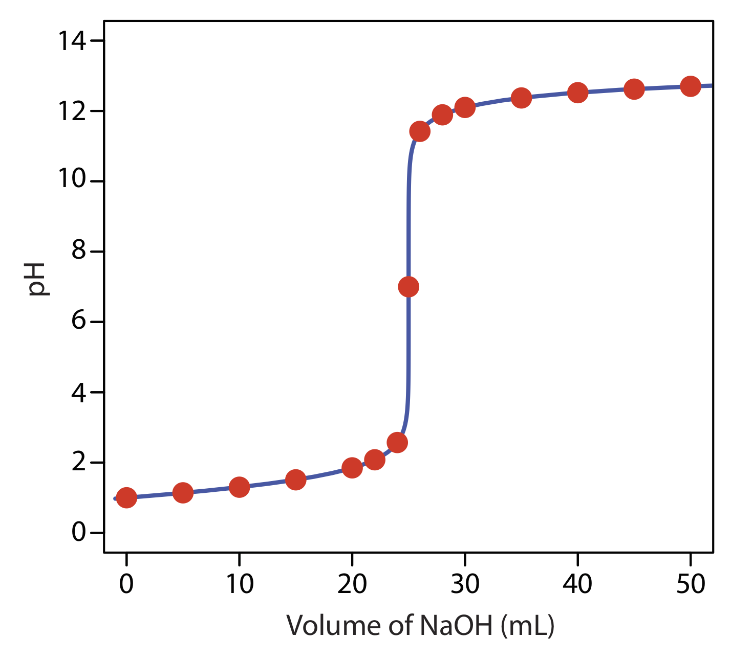
to find that the pH is 12.10. Table \(\PageIndex{1}\) and Figure \(\PageIndex{1}\) show additional results for this titration curve. You can use this same approach to calculate the titration curve for the titration of a strong base with a strong acid, except the strong base is in excess before the equivalence point and the strong acid is in excess after the equivalence point.
Construct a titration curve for the titration of 25.0 mL of 0.125 M NaOH with 0.0625 M HCl.
- Answer
-
The volume of HCl needed to reach the equivalence point is
\[V_{e q}=V_{a}=\frac{M_{b} V_{b}}{M_{a}}=\frac{(0.125 \ \mathrm{M})(25.0 \ \mathrm{mL})}{(0.0625 \ \mathrm{M})}=50.0 \ \mathrm{mL} \nonumber\]
Before the equivalence point, NaOH is present in excess and the pH is determined by the concentration of unreacted OH–. For example, after adding 10.0 mL of HCl
\[\begin{array}{c}{\left[\mathrm{OH}^{-}\right]=\frac{(0.125 \ \mathrm{M})(25.0 \ \mathrm{mL})-(0.0625 \mathrm{M})(10.0 \ \mathrm{mL})}{25.0 \ \mathrm{mL}+10.0 \ \mathrm{mL}}=0.0714 \ \mathrm{M}} \\ {\left[\mathrm{H}_{3} \mathrm{O}^{+}\right]=\frac{K_{w}}{\left[\mathrm{OH}^{-}\right]}=\frac{1.00 \times 10^{-14}}{0.0714 \ \mathrm{M}}=1.40 \times 10^{-13} \ \mathrm{M}}\end{array} \nonumber\]
the pH is 12.85.
For the titration of a strong base with a strong acid the pH at the equivalence point is 7.00.
For volumes of HCl greater than the equivalence point, the pH is determined by the concentration of excess HCl. For example, after adding 70.0 mL of titrant the concentration of HCl is
\[[\mathrm{HCl}]=\frac{(0.0625 \ \mathrm{M})(70.0 \ \mathrm{mL})-(0.125 \ \mathrm{M})(25.0 \ \mathrm{mL})}{70.0 \ \mathrm{mL}+25.0 \ \mathrm{mL}}=0.0132 \ \mathrm{M} \nonumber\]
giving a pH of 1.88. Some additional results are shown here.
volume of HCl (mL) pH volume of HCl (mL) pH 0 13.10 60 2.13 10 12.85 70 1.88 20 12.62 80 1.75 30 12.36 90 1.66 40 11.98 100 1.60 50 7.00
Titrating a Weak Acid with a Strong Base
For this example, let’s consider the titration of 50.0 mL of 0.100 M acetic acid, CH3COOH, with 0.200 M NaOH. Again, we start by calculating the volume of NaOH needed to reach the equivalence point; thus
\[\operatorname{mol} \ \mathrm{CH}_{3} \mathrm{COOH}=\mathrm{mol} \ \mathrm{NaOH} \nonumber\]
\[M_{a} \times V_{a}=M_{b} \times V_{b} \nonumber\]
\[V_{e q}=V_{b}=\frac{M_{a} V_{a}}{M_{b}}=\frac{(0.100 \ \mathrm{M})(50.0 \ \mathrm{mL})}{(0.200 \ \mathrm{M})}=25.0 \ \mathrm{mL} \nonumber\]
Before we begin the titration the pH is that for a solution of 0.100 M acetic acid. Because acetic acid is a weak acid, we calculate the pH using the method outlined in Chapter 6
\[\mathrm{CH}_{3} \mathrm{COOH}(a q)+\mathrm{H}_{2} \mathrm{O}(l)\rightleftharpoons\mathrm{H}_{3} \mathrm{O}^{+}(a q)+\mathrm{CH}_{3} \mathrm{COO}^{-}(a q) \nonumber\]
\[K_{a}=\frac{\left[\mathrm{H}_{3} \mathrm{O}^{+}\right]\left[\mathrm{CH}_{3} \mathrm{COO}^-\right]}{\left[\mathrm{CH}_{3} \mathrm{COOH}\right]}=\frac{(x)(x)}{0.100-x}=1.75 \times 10^{-5} \nonumber\]
finding that the pH is 2.88.
Adding NaOH converts a portion of the acetic acid to its conjugate base, CH3COO–.
\[\mathrm{CH}_{3} \mathrm{COOH}(a q)+\mathrm{OH}^{-}(a q) \longrightarrow \mathrm{H}_{2} \mathrm{O}(l)+\mathrm{CH}_{3} \mathrm{COO}^{-}(a q) \label{9.2}\]
Because the equilibrium constant for reaction \ref{9.2} is quite large
\[K=K_{\mathrm{a}} / K_{\mathrm{w}}=1.75 \times 10^{9} \nonumber\]
we can treat the reaction as if it goes to completion.
Any solution that contains comparable amounts of a weak acid, HA, and its conjugate weak base, A–, is a buffer. As we learned in Chapter 6, we can calculate the pH of a buffer using the Henderson–Hasselbalch equation.
\[\mathrm{pH}=\mathrm{p} K_{\mathrm{a}}+\log \frac{\left[\mathrm{A}^{-}\right]}{[\mathrm{HA}]} \nonumber\]
Before the equivalence point the concentration of unreacted acetic acid is
\[\left[\text{CH}_3\text{COOH}\right] = \frac {(\text{mol CH}_3\text{COOH})_\text{initial} - (\text{mol NaOH})_\text{added}} {\text{total volume}} = \frac {M_a V_a - M_b V_b} {V_a + V_b} \nonumber\]
and the concentration of acetate is
\[[\text{CH}_3\text{COO}^-] = \frac {(\text{mol NaOH})_\text{added}} {\text{total volume}} = \frac {M_b V_b} {V_a + V_b} \nonumber\]
For example, after adding 10.0 mL of NaOH the concentrations of CH3COOH and CH3COO– are
\[\left[\mathrm{CH}_{3} \mathrm{COOH}\right]=\frac{(0.100 \ \mathrm{M})(50.0 \ \mathrm{mL})-(0.200 \ \mathrm{M})(10.0 \ \mathrm{mL})}{50.0 \ \mathrm{mL}+10.0 \ \mathrm{mL}} = 0.0500 \text{ M} \nonumber\]
\[\left[\mathrm{CH}_{3} \mathrm{COO}^{-}\right]=\frac{(0.200 \ \mathrm{M})(10.0 \ \mathrm{mL})}{50.0 \ \mathrm{mL}+10.0 \ \mathrm{mL}}=0.0333 \ \mathrm{M} \nonumber\]
which gives us a pH of
\[\mathrm{pH}=4.76+\log \frac{0.0333 \ \mathrm{M}}{0.0500 \ \mathrm{M}}=4.58 \nonumber\]
At the equivalence point the moles of acetic acid initially present and the moles of NaOH added are identical. Because their reaction effectively proceeds to completion, the predominate ion in solution is CH3COO–, which is a weak base. To calculate the pH we first determine the concentration of CH3COO–
\[\left[\mathrm{CH}_{3} \mathrm{COO}^-\right]=\frac{(\mathrm{mol} \ \mathrm{NaOH})_{\mathrm{added}}}{\text { total volume }}= \frac{(0.200 \ \mathrm{M})(25.0 \ \mathrm{mL})}{50.0 \ \mathrm{mL}+25.0 \ \mathrm{mL}}=0.0667 \ \mathrm{M} \nonumber\]
Alternatively, we can calculate acetate’s concentration using the initial moles of acetic acid; thus
\[\left[\mathrm{CH}_{3} \mathrm{COO}^{-}\right]=\frac{\left(\mathrm{mol} \ \mathrm{CH}_{3} \mathrm{COOH}\right)_{\mathrm{initial}}}{\text { total volume }} = \frac{(0.100 \ \mathrm{M})(50.0 \ \mathrm{mL})}{50.0 \ \mathrm{mL}+25.0 \ \mathrm{mL}} = 0.0667 \text{ M} \nonumber\]
Next, we calculate the pH of the weak base as shown earlier in Chapter 6
\[\mathrm{CH}_{3} \mathrm{COO}^{-}(a q)+\mathrm{H}_{2} \mathrm{O}(l)\rightleftharpoons\mathrm{OH}^{-}(a q)+\mathrm{CH}_{3} \mathrm{COOH}(a q) \nonumber\]
\[K_{\mathrm{b}}=\frac{\left[\mathrm{OH}^{-}\right]\left[\mathrm{CH}_{3} \mathrm{COOH}\right]}{\left[\mathrm{CH}_{3} \mathrm{COO}^{-}\right]}=\frac{(x)(x)}{0.0667-x}=5.71 \times 10^{-10} \nonumber\]
\[x=\left[\mathrm{OH}^{-}\right]=6.17 \times 10^{-6} \ \mathrm{M} \nonumber\]
\[\left[\mathrm{H}_{3} \mathrm{O}^{+}\right]=\frac{K_{\mathrm{w}}}{\left[\mathrm{OH}^{-}\right]}=\frac{1.00 \times 10^{-14}}{6.17 \times 10^{-6}}=1.62 \times 10^{-9} \ \mathrm{M} \nonumber\]
finding that the pH at the equivalence point is 8.79.
After the equivalence point, the titrant is in excess and the titration mixture is a dilute solution of NaOH. We can calculate the pH using the same strategy as in the titration of a strong acid with a strong base. For example, after adding 30.0 mL of NaOH the concentration of OH– is
\[\left[\mathrm{OH}^{-}\right]=\frac{(0.200 \ \mathrm{M})(30.0 \ \mathrm{mL})-(0.100 \ \mathrm{M})(50.0 \ \mathrm{mL})}{30.0 \ \mathrm{mL}+50.0 \ \mathrm{mL}}=0.0125 \ \mathrm{M} \nonumber\]
\[\left[\mathrm{H}_{3} \mathrm{O}^{+}\right]=\frac{K_{\mathrm{w}}}{\left[\mathrm{OH}^{-}\right]}=\frac{1.00 \times 10^{-14}}{0.0125}=8.00 \times 10^{-13} \ \mathrm{M} \nonumber\]
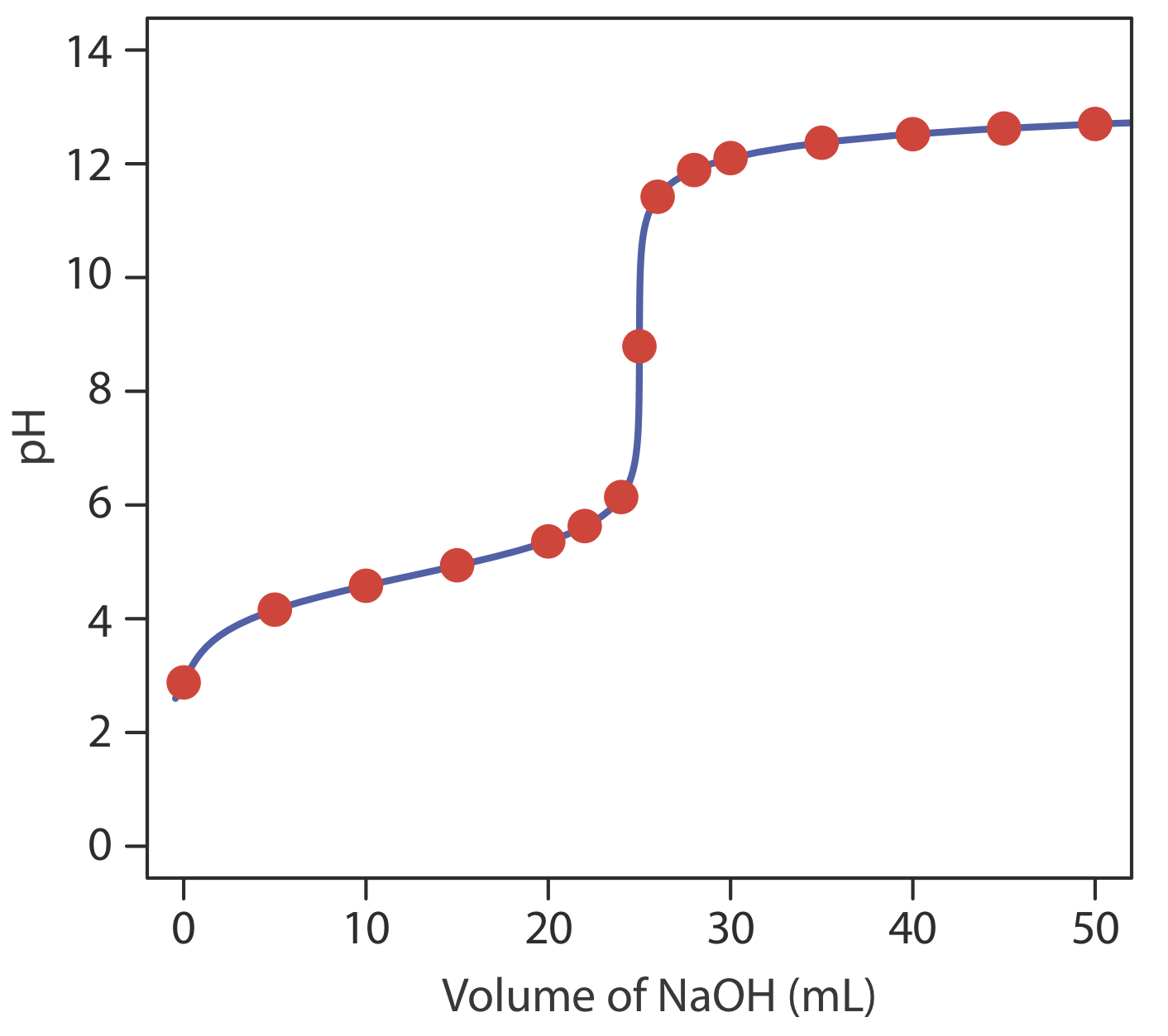
giving a pH of 12.10. Table \(\PageIndex{2}\) and Figure \(\PageIndex{2}\) show additional results for this titration. You can use this same approach to calculate the titration curve for the titration of a weak base with a strong acid, except the initial pH is determined by the weak base, the pH at the equivalence point by its conjugate weak acid, and the pH after the equivalence point by excess strong acid.
Construct a titration curve for the titration of 25.0 mL of 0.125 M NH3 with 0.0625 M HCl.
- Answer
-
The volume of HCl needed to reach the equivalence point is
\[V_{a q}=V_{a}=\frac{M_{b} V_{b}}{M_{a}}=\frac{(0.125 \ \mathrm{M})(25.0 \ \mathrm{mL})}{(0.0625 \ \mathrm{M})}=50.0 \ \mathrm{mL} \nonumber\]
Before adding HCl the pH is that for a solution of 0.100 M NH3.
\[K_{\mathrm{b}}=\frac{[\mathrm{OH}^-]\left[\mathrm{NH}_{4}^{+}\right]}{\left[\mathrm{NH}_{3}\right]}=\frac{(x)(x)}{0.125-x}=1.75 \times 10^{-5} \nonumber\]
\[x=\left[\mathrm{OH}^{-}\right]=1.48 \times 10^{-3} \ \mathrm{M} \nonumber\]
\[\left[\mathrm{H}_{3} \mathrm{O}^{+}\right]=\frac{K_{\mathrm{w}}}{[\mathrm{OH}^-]}=\frac{1.00 \times 10^{-14}}{1.48 \times 10^{-3} \ \mathrm{M}}=6.76 \times 10^{-12} \ \mathrm{M} \nonumber\]
The pH at the beginning of the titration, therefore, is 11.17.
Before the equivalence point the pH is determined by an \(\text{NH}_3/\text{NH}_4^+\) buffer. For example, after adding 10.0 mL of HCl
\[\left[\mathrm{NH}_{3}\right]=\frac{(0.125 \ \mathrm{M})(25.0 \ \mathrm{mL})-(0.0625 \ \mathrm{M})(10.0 \ \mathrm{mL})}{25.0 \ \mathrm{mL}+10.0 \ \mathrm{mL}}=0.0714 \ \mathrm{M} \nonumber\]
\[\left[\mathrm{NH}_{4}^{+}\right]=\frac{(0.0625 \ \mathrm{M})(10.0 \ \mathrm{mL})}{25.0 \ \mathrm{mL}+10.0 \ \mathrm{mL}}=0.0179 \ \mathrm{M} \nonumber\]
\[\mathrm{pH}=9.244+\log \frac{0.0714 \ \mathrm{M}}{0.0179 \ \mathrm{M}}=9.84 \nonumber\]
At the equivalence point the predominate ion in solution is \(\text{NH}_4^+\) . To calculate the pH we first determine the concentration of \(\text{NH}_4^+\)
\[\left[\mathrm{NH}_{4}^{+}\right]=\frac{(0.125 \ \mathrm{M})(25.0 \ \mathrm{mL})}{25.0 \ \mathrm{mL}+50.0 \ \mathrm{mL}}=0.0417 \ \mathrm{M} \nonumber\]
and then calculate the pH
\[K_{\mathrm{a}}=\frac{\left[\mathrm{H}_{3} \mathrm{O}^{+}\right]\left[\mathrm{NH}_{3}\right]}{\left[\mathrm{NH}_{4}^{+}\right]}=\frac{(x)(x)}{0.0417-x}=5.70 \times 10^{-10} \nonumber\]
obtaining a value of 5.31.
After the equivalence point, the pH is determined by the excess HCl. For example, after adding 70.0 mL of HCl
\[[\mathrm{HCl}]=\frac{(0.0625 \ \mathrm{M})(70.0 \ \mathrm{mL})-(0.125 \ \mathrm{M})(25.0 \ \mathrm{mL})}{70.0 \ \mathrm{mL}+25.0 \ \mathrm{mL}}=0.0132 \ \mathrm{M} \nonumber\]
and the pH is 1.88. Some additional results are shown here.
volume of HCl (mL) pH volume of HCl (mL) pH 0 11.17 60 2.13 10 9.84 70 1.88 20 9.42 80 1.75 30 9.07 90 1.66 40 8.64 100 1.60 50 5.31
We can extend this approach for calculating a weak acid–strong base titration curve to reactions that involve multiprotic acids or bases, and mixtures of acids or bases. As the complexity of the titration increases, however, the necessary calculations become more time consuming. Not surprisingly, a variety of algebraic and spreadsheet approaches are available to aid in constructing titration curves.
The following papers provide information on algebraic approaches to calculating titration curves: (a) Willis, C. J. J. Chem. Educ. 1981, 58, 659–663; (b) Nakagawa, K. J. Chem. Educ. 1990, 67, 673–676; (c) Gordus, A. A. J. Chem. Educ. 1991, 68, 759–761; (d) de Levie, R. J. Chem. Educ. 1993, 70, 209–217; (e) Chaston, S. J. Chem. Educ. 1993, 70, 878–880; (f) de Levie, R. Anal. Chem. 1996, 68, 585–590.
The following papers provide information on the use of spreadsheets to generate titration curves: (a) Currie, J. O.; Whiteley, R. V. J. Chem. Educ. 1991, 68, 923–926; (b) Breneman, G. L.; Parker, O. J. J. Chem. Educ. 1992, 69, 46–47; (c) Carter, D. R.; Frye, M. S.; Mattson, W. A. J. Chem. Educ. 1993, 70, 67–71; (d) Freiser, H. Concepts and Calculations in Analytical Chemistry, CRC Press: Boca Raton, 1992.
Sketching an Acid–Base Titration Curve
To evaluate the relationship between a titration’s equivalence point and its end point we need to construct only a reasonable approximation of the exact titration curve. In this section we demonstrate a simple method for sketching an acid–base titration curve. Our goal is to sketch the titration curve quickly, using as few calculations as possible. Let’s use the titration of 50.0 mL of 0.100 M CH3COOH with 0.200 M NaOH to illustrate our approach. This is the same example that we used to develop the calculations for a weak acid–strong base titration curve. You can review the results of that calculation in Table \(\PageIndex{2}\) and in Figure \(\PageIndex{2}\).
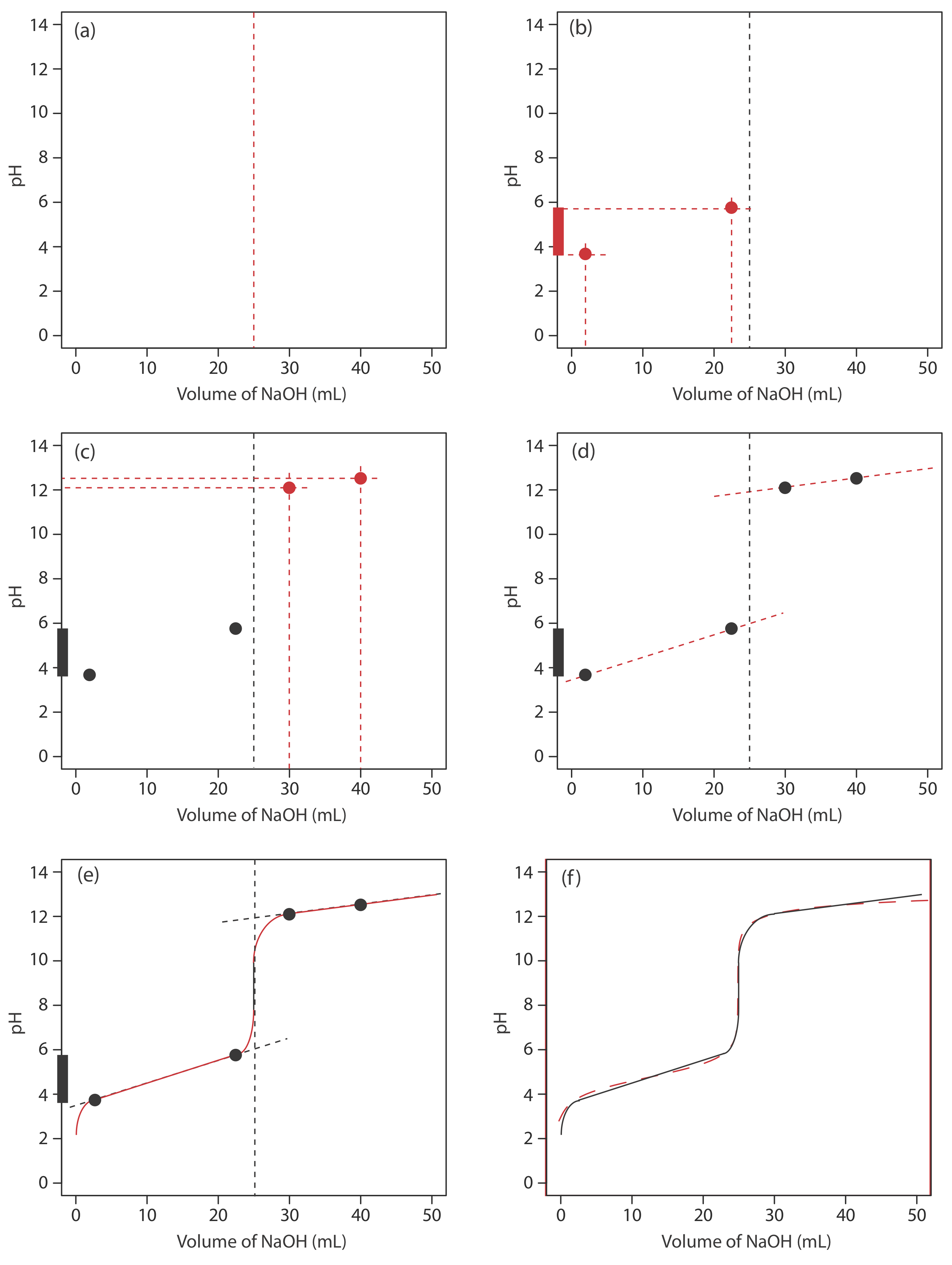
We begin by calculating the titration’s equivalence point volume, which, as we determined earlier, is 25.0 mL. Next we draw our axes, placing pH on the y-axis and the titrant’s volume on the x-axis. To indicate the equivalence point volume, we draw a vertical line that intersects the x-axis at 25.0 mL of NaOH. Figure \(\PageIndex{3}\)a shows the first step in our sketch.
Before the equivalence point the titrand’s pH is determined by a buffer of acetic acid, CH3COOH, and acetate, CH3COO–. Although we can calculate a buffer’s pH using the Henderson–Hasselbalch equation, we can avoid this calculation by making a simple assumption. You may recall from Chapter 6 that a buffer operates over a pH range that extends approximately ±1 pH unit on either side of the weak acid’s pKa value. The pH is at the lower end of this range, pH = pKa – 1, when the weak acid’s concentration is \(10 \times\) greater than that of its conjugate weak base. The buffer reaches its upper pH limit, pH = pKa + 1, when the weak acid’s concentration is \(10 \times\) smaller than that of its conjugate weak base. When we titrate a weak acid or a weak base, the buffer spans a range of volumes from approximately 10% of the equivalence point volume to approximately 90% of the equivalence point volume.
The actual values are 9.09% and 90.9%, but for our purpose, using 10% and 90% is more convenient; that is, after all, one advantage of an approximation!
Figure \(\PageIndex{3}\)b shows the second step in our sketch. First, we superimpose acetic acid’s ladder diagram on the y-axis, including its buffer range, using its pKa value of 4.76. Next, we add two points, one for the pH at 10% of the equivalence point volume (a pH of 3.76 at 2.5 mL) and one for the pH at 90% of the equivalence point volume (a pH of 5.76 at 22.5 mL).
The third step is to add two points after the equivalence point. The pH after the equivalence point is fixed by the concentration of excess titrant, NaOH. Calculating the pH of a strong base is straightforward, as we saw earlier. Figure \(\PageIndex{3}\)c includes points (see Table \(\PageIndex{2}\)) for the pH after adding 30.0 mL and after adding 40.0 mL of NaOH.
Next, we draw a straight line through each pair of points, extending each line through the vertical line that represents the equivalence point’s volume (Figure \(\PageIndex{3}\)d). Finally, we complete our sketch by drawing a smooth curve that connects the three straight-line segments (Figure \(\PageIndex{3}\)e). A comparison of our sketch to the exact titration curve (Figure \(\PageIndex{3}\)f) shows that they are in close agreement.
Sketch a titration curve for the titration of 25.0 mL of 0.125 M NH3 with 0.0625 M HCl and compare to the result from Exercise \(\PageIndex{2}\).
- Answer
-
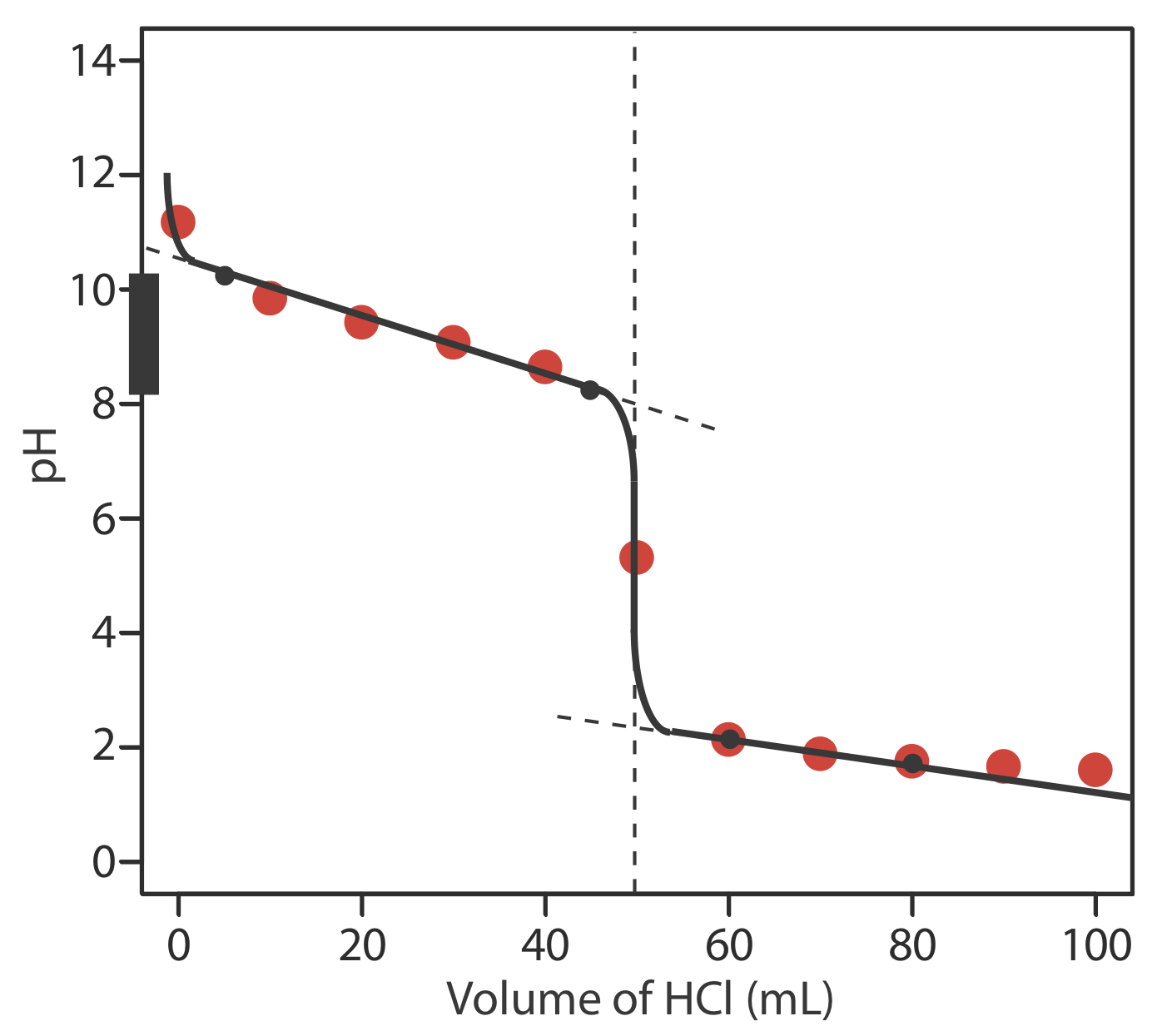
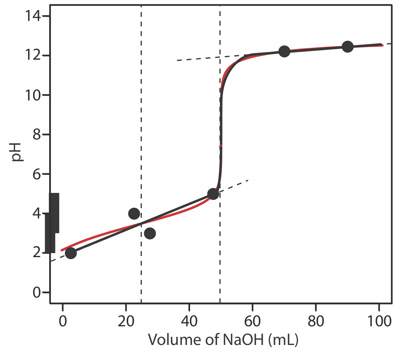
The figure below shows a sketch of the titration curve. The black dots and curve are the approximate sketch of the titration curve. The points in red are the calculations from Exercise \(\PageIndex{2}\). The two black points before the equivalence point (VHCl = 5 mL, pH = 10.24 and VHCl = 45 mL, pH= 8.24) are plotted using the pKa of 9.244 for \(\text{NH}_4^+\). The two black points after the equivalence point (VHCl = 60 mL, pH = 2.13 and VHCl = 80 mL, pH= 1.75 ) are from the answer to Exercise \(\PageIndex{2}\).
As shown in the following example, we can adapt this approach to any acid–base titration, including those where exact calculations are more challenging, including the titration of polyprotic weak acids and bases, and the titration of mixtures of weak acids or weak bases.
Sketch titration curves for the following two systems: (a) the titration of 50.0 mL of 0.050 M H2A, a diprotic weak acid with a pKa1 of 3 and a pKa2 of 7; and (b) the titration of a 50.0 mL mixture that contains 0.075 M HA, a weak acid with a pKa of 3, and 0.025 M HB, a weak acid with a pKa of 7. For both titrations, assume that the titrant is 0.10 M NaOH.
Solution
Figure \(\PageIndex{4}\)a shows the titration curve for H2A, including the ladder diagram for H2A on the y-axis, the two equivalence points at 25.0 mL and at 50.0 mL, two points before each equivalence point, two points after the last equivalence point, and the straight-lines used to sketch the final titration curve. Before the first equivalence point the pH is controlled by a buffer of H2A and HA–. An HA–/A2– buffer controls the pH between the two equivalence points. After the second equivalence point the pH reflects the concentration of excess NaOH.
Figure \(\PageIndex{4}\)b shows the titration curve for the mixture of HA and HB. Again, there are two equivalence points; however, in this case the equivalence points are not equally spaced because the concentration of HA is greater than that for HB. Because HA is the stronger of the two weak acids it reacts first; thus, the pH before the first equivalence point is controlled by a buffer of HA and A–. Between the two equivalence points the pH reflects the titration of HB and is determined by a buffer of HB and B–. After the second equivalence point excess NaOH determines the pH.

Sketch the titration curve for 50.0 mL of 0.050 M H2A, a diprotic weak acid with a pKa1 of 3 and a pKa2 of 4, using 0.100 M NaOH as the titrant. The fact that pKa2 falls within the buffer range of pKa1 presents a challenge that you will need to consider.
- Answer
-
The figure below shows a sketch of the titration curve. The titration curve has two equivalence points, one at 25.0 mL \((\text{H}_2\text{A} \rightarrow \text{HA}^-)\) and one at 50.0 mL (\(\text{HA}^- \rightarrow \text{A}^{2-}\)). In sketching the curve, we plot two points before the first equivalence point using the pKa1 of 3 for H2A
\[V_{\mathrm{HCl}}=2.5 \ \mathrm{mL}, \mathrm{pH}=2 \text { and } V_{\mathrm{HCl}}=22.5 \ \mathrm{mL}, \mathrm{pH}=4 \nonumber\]
two points between the equivalence points using the pKa2 of 5 for HA–
\[V_{\mathrm{HCl}}=27.5 \ \mathrm{mL}, \mathrm{pH}=3, \text { and } V_{\mathrm{HCl}}=47.5 \ \mathrm{mL}, \mathrm{pH}=5 \nonumber\]
and two points after the second equivalence point
\[V_{\mathrm{HCl}}=70 \ \mathrm{mL}, \mathrm{pH}=12.22 \text { and } V_{\mathrm{HCl}}=90 \ \mathrm{mL}, \mathrm{pH}=12.46 \nonumber\]
Drawing a smooth curve through these points presents us with the following dilemma—the pH appears to increase as the titrant’s volume approaches the first equivalence point and then appears to decrease as it passes through the first equivalence point. This is, of course, absurd; as we add NaOH the pH cannot decrease. Instead, we model the titration curve before the second equivalence point by drawing a straight line from the first point (VHCl = 2.5 mL, pH = 2) to the fourth point (VHCl = 47.5 mL, pH= 5), ignoring the second and third points. The results is a reasonable approximation of the exact titration curve.
Selecting and Evaluating the End Point
Earlier we made an important distinction between a titration’s end point and its equivalence point. The difference between these two terms is important and deserves repeating. An equivalence point, which occurs when we react stoichiometrically equal amounts of the analyte and the titrant, is a theoretical not an experimental value. A titration’s end point is an experimental result that represents our best estimate of the equivalence point. Any difference between a titration’s equivalence point and its corresponding end point is a source of determinate error.
Where is the Equivalence Point?
Earlier we learned how to calculate the pH at the equivalence point for the titration of a strong acid with a strong base, and for the titration of a weak acid with a strong base. We also learned how to sketch a titration curve with only a minimum of calculations. Can we also locate the equivalence point without performing any calculations. The answer, as you might guess, often is yes!
For most acid–base titrations the inflection point—the point on a titration curve that has the greatest slope—very nearly coincides with the titration’s equivalence point. The red arrows in Figure \(\PageIndex{4}\), for example, identify the equivalence points for the titration curves in Example \(\PageIndex{1}\). An inflection point actually precedes its corresponding equivalence point by a small amount, with the error approaching 0.1% for weak acids and weak bases with dissociation constants smaller than 10–9, or for very dilute solutions [Meites, L.; Goldman, J. A. Anal. Chim. Acta 1963, 29, 472–479].
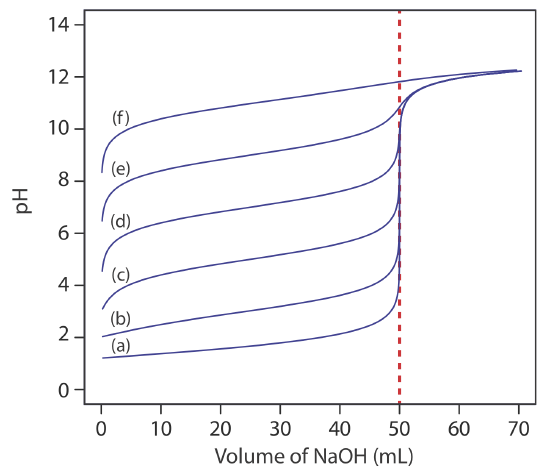
The principal limitation of an inflection point is that it must be present and easy to identify. For some titrations the inflection point is missing or difficult to find. Figure \(\PageIndex{5}\), for example, demonstrates the affect of a weak acid’s dissociation constant, Ka, on the shape of its titration curve. An inflection point is visible, even if barely so, for acid dissociation constants larger than 10–9, but is missing when Ka is 10–11.
An inflection point also may be missing or difficult to see if the analyte is a multiprotic weak acid or weak base with successive dissociation constants that are similar in magnitude. To appreciate why this is true let’s consider the titration of a diprotic weak acid, H2A, with NaOH. During the titration the following two reactions occur.
\[\mathrm{H}_{2} \mathrm{A}(a q)+\mathrm{OH}^{-}(a q) \longrightarrow \mathrm{H}_{2} \mathrm{O}(l)+\mathrm{HA}^{-}(a q) \label{9.3}\]
\[\mathrm{HA}^{-}(a q)+\mathrm{OH}^{-}(a q) \rightarrow \mathrm{H}_{2} \mathrm{O}(l)+\mathrm{A}^{2-}(a q) \label{9.4}\]
To see two distinct inflection points, reaction \ref{9.3} must essentially be complete before reaction \ref{9.4} begins.
Figure \(\PageIndex{6}\) shows titration curves for three diprotic weak acids. The titration curve for maleic acid, for which Ka1 is approximately \(20000 \times\) larger than Ka2, has two distinct inflection points. Malonic acid, on the other hand, has acid dissociation constants that differ by a factor of approximately 690. Although malonic acid’s titration curve shows two inflection points, the first is not as distinct as the second. Finally, the titration curve for succinic acid, for which the two Ka values differ by a factor of only \(27 \times\), has only a single inflection point that corresponds to the neutralization of \(\text{HC}_2\text{H}_4\text{O}_4^-\) to \(\text{C}_2\text{H}_4\text{O}_4^{2-}\). In general, we can detect separate inflection points when successive acid dissociation constants differ by a factor of at least 500 (a \(\Delta\)Ka of at least 2.7).

The same holds true for mixtures of weak acids or mixtures of weak bases. To detect separate inflection points when titrating a mixture of weak acids, their pKa values must differ by at least a factor of 500.
Finding the End Point with an Indicator
One interesting group of weak acids and weak bases are organic dyes. Because an organic dye has at least one highly colored conjugate acid–base species, its titration results in a change in both its pH and its color. We can use this change in color to indicate the end point of a titration provided that it occurs at or near the titration’s equivalence point.
As an example, let’s consider an indicator for which the acid form, HIn, is yellow and the base form, In–, is red. The color of the indicator’s solution depends on the relative concentrations of HIn and In–. To understand the relationship between pH and color we use the indicator’s acid dissociation reaction
\[\mathrm{HIn}(a q)+\mathrm{H}_{2} \mathrm{O}(l)\rightleftharpoons \mathrm{H}_{3} \mathrm{O}^{+}(a q)+\operatorname{In}^{-}(a q) \nonumber\]
and its equilibrium constant expression.
\[K_{\mathrm{a}}=\frac{\left[\mathrm{H}_{3} \mathrm{O}^{+}\right]\left[\mathrm{In}^{-}\right]}{[\mathrm{HIn}]} \label{9.5}\]
Taking the negative log of each side of equation \ref{9.5}, and rearranging to solve for pH leaves us with a equation that relates the solution’s pH to the relative concentrations of HIn and In–.
\[\mathrm{pH}=\mathrm{p} K_{\mathrm{a}}+\log \frac{[\mathrm{In}^-]}{[\mathrm{HIn}]} \label{9.6}\]
If we can detect HIn and In– with equal ease, then the transition from yellow-to-red (or from red-to-yellow) reaches its midpoint, which is orange, when the concentrations of HIn and In– are equal, or when the pH is equal to the indicator’s pKa. If the indicator’s pKa and the pH at the equivalence point are identical, then titrating until the indicator turns orange is a suitable end point. Unfortunately, we rarely know the exact pH at the equivalence point. In addition, determining when the concentrations of HIn and In– are equal is difficult if the indicator’s change in color is subtle.
We can establish the range of pHs over which the average analyst observes a change in the indicator’s color by making two assumptions: that the indicator’s color is yellow if the concentration of HIn is \(10 \times\) greater than that of In– and that its color is red if the concentration of HIn is \(10 \times\) smaller than that of In–. Substituting these inequalities into equation \ref{9.6}
\[\begin{array}{l}{\mathrm{pH}=\mathrm{p} K_{\mathrm{a}}+\log \frac{1}{10}=\mathrm{p} K_{\mathrm{a}}-1} \\ {\mathrm{pH}=\mathrm{p} K_{\mathrm{a}}+\log \frac{10}{1}=\mathrm{p} K_{\mathrm{a}}+1}\end{array} \nonumber\]
shows that the indicator changes color over a pH range that extends ±1 unit on either side of its pKa. As shown in Figure \(\PageIndex{7}\), the indicator is yel-ow when the pH is less than pKa – 1 and it is red when the pH is greater than pKa + 1. For pH values between pKa – 1 and pKa + 1 the indicator’s color passes through various shades of orange. The properties of several common acid–base indicators are listed in Table \(\PageIndex{3}\).
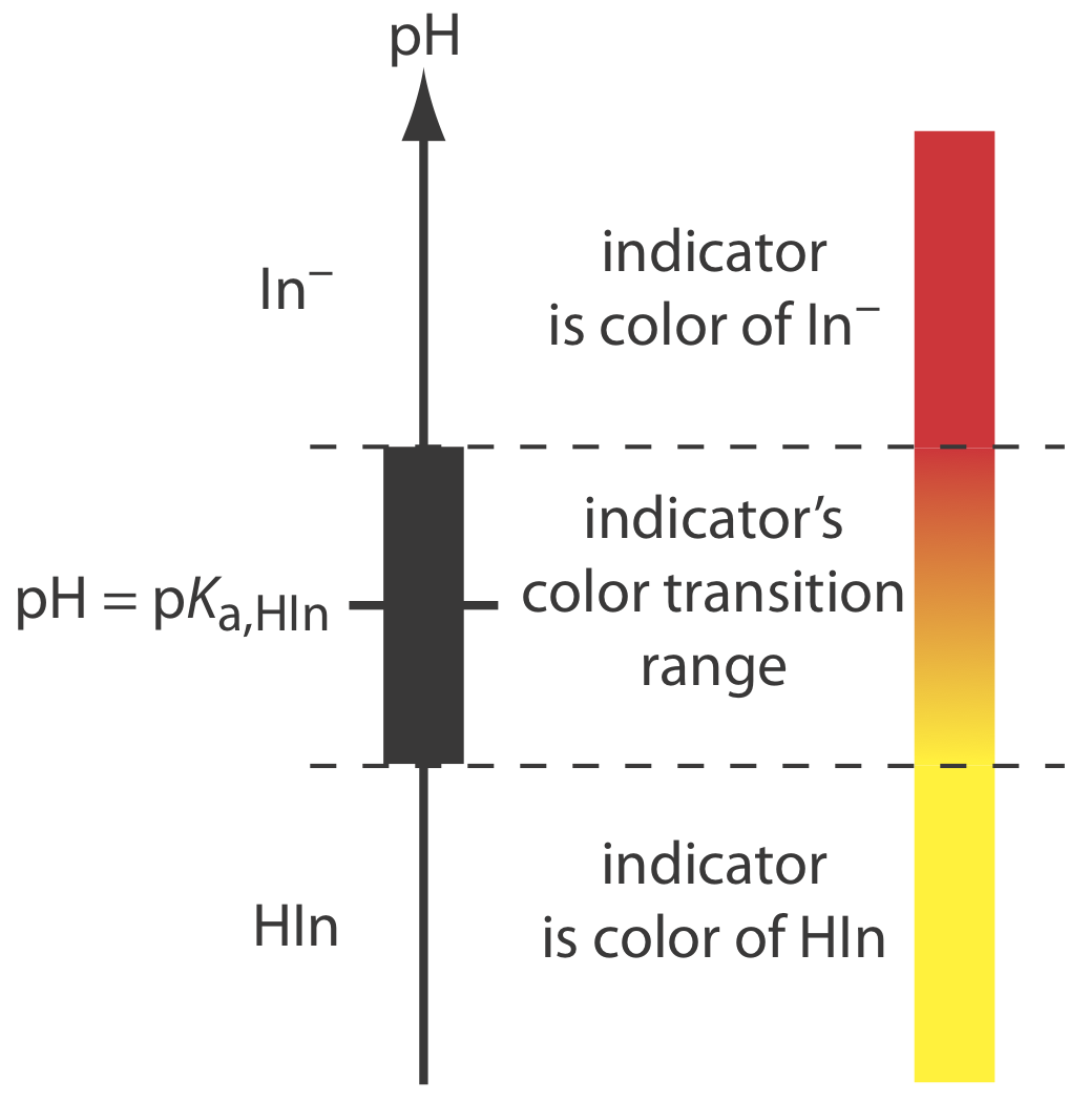
You may wonder why an indicator’s pH range, such as that for phenolphthalein, is not equally distributed around its pKa value. The explanation is simple. Figure \(\PageIndex{7}\) presents an idealized view in which our sensitivity to the indicator’s two colors is equal. For some indicators only the weak acid or the weak base is colored. For other indicators both the weak acid and the weak base are colored, but one form is easier to see. In either case, the indicator’s pH range is skewed in the direction of the indicator’s less colored form. Thus, phenolphthalein’s pH range is skewed in the direction of its colorless form, shifting the pH range to values lower than those suggested by Figure \(\PageIndex{7}\).
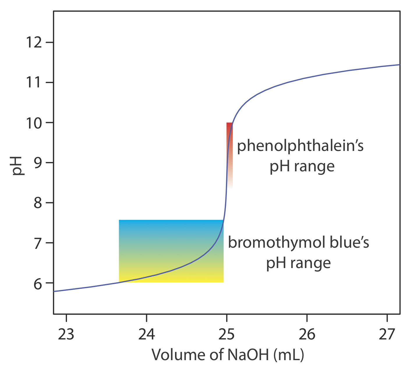
The relatively broad range of pHs over which an indicator changes color places additional limitations on its ability to signal a titration’s end point. To minimize a determinate titration error, the indicator’s entire pH range must fall within the rapid change in pH near the equivalence point. For example, in Figure \(\PageIndex{8}\) we see that phenolphthalein is an appropriate indicator for the titration of 50.0 mL of 0.050 M acetic acid with 0.10 M NaOH. Bromothymol blue, on the other hand, is an inappropriate indicator because its change in color begins well before the initial sharp rise in pH, and, as a result, spans a relatively large range of volumes. The early change in color increases the probability of obtaining an inaccurate result, and the range of possible end point volumes increases the probability of obtaining imprecise results.
Suggest a suitable indicator for the titration of 25.0 mL of 0.125 M NH3 with 0.0625 M NaOH. You constructed a titration curve for this titration in Exercise \(\PageIndex{2}\) and Exercise \(\PageIndex{3}\).
- Answer
-
The pH at the equivalence point is 5.31 (see Exercise \(\PageIndex{2}\)) and the sharp part of the titration curve extends from a pH of approximately 7 to a pH of approximately 4. Of the indicators in Table \(\PageIndex{3}\), methyl red is the best choice because its pKa value of 5.0 is closest to the equivalence point’s pH and because the pH range of 4.2–6.3 for its change in color will not produce a significant titration error.
Finding the End Point by Monitoring pH
An alternative approach for locating a titration’s end point is to monitor the titration’s progress using a sensor whose signal is a function of the analyte’s concentration. The result is a plot of the entire titration curve, which we can use to locate the end point with a minimal error.
A pH electrode is the obvious sensor for monitoring an acid–base titration and the result is a potentiometric titration curve. For example, Figure \(\PageIndex{9}\)a shows a small portion of the potentiometric titration curve for the titration of 50.0 mL of 0.050 M CH3COOH with 0.10 M NaOH, which focuses on the region that contains the equivalence point. The simplest method for finding the end point is to locate the titration curve’s inflection point, which is shown by the arrow. This is also the least accurate method, particularly if the titration curve has a shallow slope at the equivalence point.
See Chapter 11 for more details about pH electrodes.
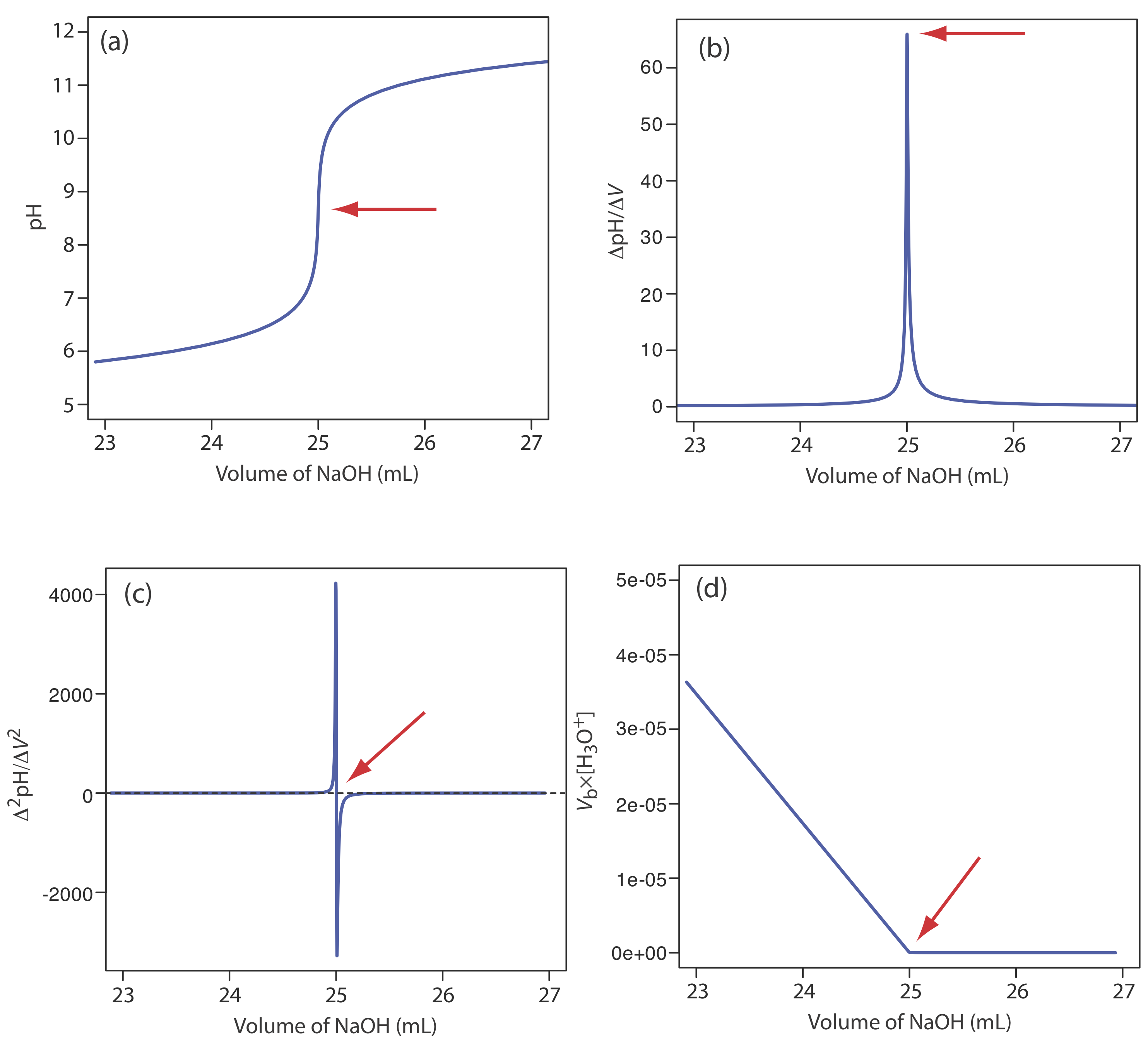
Another method for locating the end point is to plot the first derivative of the titration curve, which gives its slope at each point along the x-axis. Examine Figure \(\PageIndex{9}\)a and consider how the titration curve’s slope changes as we approach, reach, and pass the equivalence point. Because the slope reaches its maximum value at the inflection point, the first derivative shows a spike at the equivalence point (Figure \(\PageIndex{9}\)b). The second derivative of a titration curve can be more useful than the first derivative because the equivalence point intersects the volume axis. Figure \(\PageIndex{9}\)c shows the resulting titration curve.
Suppose we have the following three points on our titration curve:
| volume (mL) | pH |
| 23.65 | 6.00 |
| 23.91 | 6.10 |
| 24.13 | 6.20 |
Mathematically, we can approximate the first derivative as \(\Delta \text{pH} / \Delta V\), where \(\Delta \text{pH}\) is the change in pH between successive additions of titrant. Using the first two points, the first derivative is
\[\frac{\Delta \mathrm{pH}}{\Delta V}=\frac{6.10-6.00}{23.91-23.65}=0.385 \nonumber\]
which we assign to the average of the two volumes, or 23.78 mL. For the second and third points, the first derivative is 0.455 and the average volume is 24.02 mL.
| volume (mL) | \(\Delta \text{pH}\) |
| 23.78 | 0.385 |
| 24.02 | 0.455 |
We can approximate the second derivative as \(\Delta (\Delta \text{pH} / \Delta V) / \Delta V\), or \(\Delta^2 \text{pH} / \Delta V^2\). Using the two points from our calculation of the first derivative, the second derivative is
\[\frac{\Delta^{2} \mathrm{p} \mathrm{H}}{\Delta V^{2}}=\frac{0.455-0.385}{24.02-23.78}=0.292 \nonumber\]
which we assign to the average of the two volumes, or 23.90 mL. Note that calculating the first derivative comes at the expense of losing one piece of information (three points become two points), and calculating the second derivative comes at the expense of losing two pieces of information.
Derivative methods are particularly useful when titrating a sample that contains more than one analyte. If we rely on indicators to locate the end points, then we usually must complete separate titrations for each analyte so that we can see the change in color for each end point. If we record the titration curve, however, then a single titration is sufficient. The precision with which we can locate the end point also makes derivative methods attractive for an analyte that has a poorly defined normal titration curve.
Derivative methods work well only if we record sufficient data during the rapid increase in pH near the equivalence point. This usually is not a problem if we use an automatic titrator, such as the one seen earlier in Figure 9.1.5. Because the pH changes so rapidly near the equivalence point—a change of several pH units over a span of several drops of titrant is not unusual—a manual titration does not provide enough data for a useful derivative titration curve. A manual titration does contain an abundance of data during the more gently rising portions of the titration curve before and after the equivalence point. This data also contains information about the titration curve’s equivalence point.
Consider again the titration of acetic acid, CH3COOH, with NaOH. At any point during the titration acetic acid is in equilibrium with H3O+ and CH3COO–
\[\mathrm{CH}_{3} \mathrm{COOH}(a q)+\mathrm{H}_{2} \mathrm{O}(l )\rightleftharpoons\mathrm{H}_{3} \mathrm{O}^{+}(a q)+\mathrm{CH}_{3} \mathrm{COO}^{-}(a q) \nonumber\]
for which the equilibrium constant is
\[K_{a}=\frac{\left[\mathrm{H}_{3} \mathrm{O}^{+}\right]\left[\mathrm{CH}_{3} \mathrm{COO}^{-}\right]}{\left[\mathrm{CH}_{3} \mathrm{COOH}\right]} \nonumber\]
Before the equivalence point the concentrations of CH3COOH and CH3COO– are
\[[\text{CH}_3\text{COOH}] = \frac {(\text{mol CH}_3\text{COOH})_\text{initial} - (\text{mol NaOH})_\text{added}} {\text{total volume}} = \frac {M_a V_a - M_b V_b} {V_a + V_b} \nonumber\]
\[[\text{CH}_3\text{COO}^-] = \frac {(\text{mol NaOH})_\text{added}} {\text{total volume}} = \frac {M_b V_b} {V_a + V_b} \nonumber\]
Substituting these equations into the Ka expression and rearranging leaves us with
\[K_{\mathrm{a}}=\frac{\left[\mathrm{H}_{3} \mathrm{O}^{+}\right]\left(M_{b} V_{b}\right) /\left(V_{a}+V_{b}\right)}{\left\{M_{a} V_{a}-M_{b} V_{b}\right\} /\left(V_{a}+V_{b}\right)} \nonumber\]
\[K_{a} M_{a} V_{a}-K_{a} M_{b} V_{b}=\left[\mathrm{H}_{3} \mathrm{O}^{+}\right]\left(M_{b} V_{b}\right) \nonumber\]
\[\frac{K_{a} M_{a} V_{a}}{M_{b}}-K_{a} V_{b}=\left[\mathrm{H}_{3} \mathrm{O}^{+}\right] V_{b} \nonumber\]
Finally, recognizing that the equivalence point volume is
\[V_{eq}=\frac{M_{a} V_{a}}{M_{b}} \nonumber\]
leaves us with the following equation.
\[\left[\mathrm{H}_{3} \mathrm{O}^{+}\right] \times V_{b}=K_{\mathrm{a}} V_{eq}-K_{\mathrm{a}} V_{b} \nonumber\]
For volumes of titrant before the equivalence point, a plot of \(V_b \times [\text{H}_3\text{O}^+]\) versus Vb is a straight-line with an x-intercept of Veq and a slope of –Ka. Figure \(\PageIndex{9}\)d shows a typical result. This method of data analysis, which converts a portion of a titration curve into a straight-line, is a Gran plot.
Values of Ka determined by this method may have a substantial error if the effect of activity is ignored. See Chapter 6.9 for a discussion of activity.
Finding the End Point by Monitoring Temperature
The reaction between an acid and a base is exothermic. Heat generated by the reaction is absorbed by the titrand, which increases its temperature. Monitoring the titrand’s temperature as we add the titrant provides us with another method for recording a titration curve and identifying the titration’s end point (Figure \(\PageIndex{10}\)).
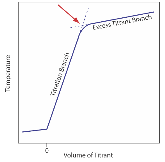
Before we add the titrant, any change in the titrand’s temperature is the result of warming or cooling as it equilibrates with the surroundings. Adding titrant initiates the exothermic acid–base reaction and increases the titrand’s temperature. This part of a thermometric titration curve is called the titration branch. The temperature continues to rise with each addition of titrant until we reach the equivalence point. After the equivalence point, any change in temperature is due to the titrant’s enthalpy of dilution and the difference between the temperatures of the titrant and titrand. Ideally, the equivalence point is a distinct intersection of the titration branch and the excess titrant branch. As shown in Figure \(\PageIndex{10}\), however, a thermometric titration curve usually shows curvature near the equivalence point due to an incomplete neutralization reaction or to the excessive dilution of the titrand and the titrant during the titration. The latter problem is minimized by using a titrant that is 10–100 times more concentrated than the analyte, although this results in a very small end point volume and a larger relative error. If necessary, the end point is found by extrapolation.
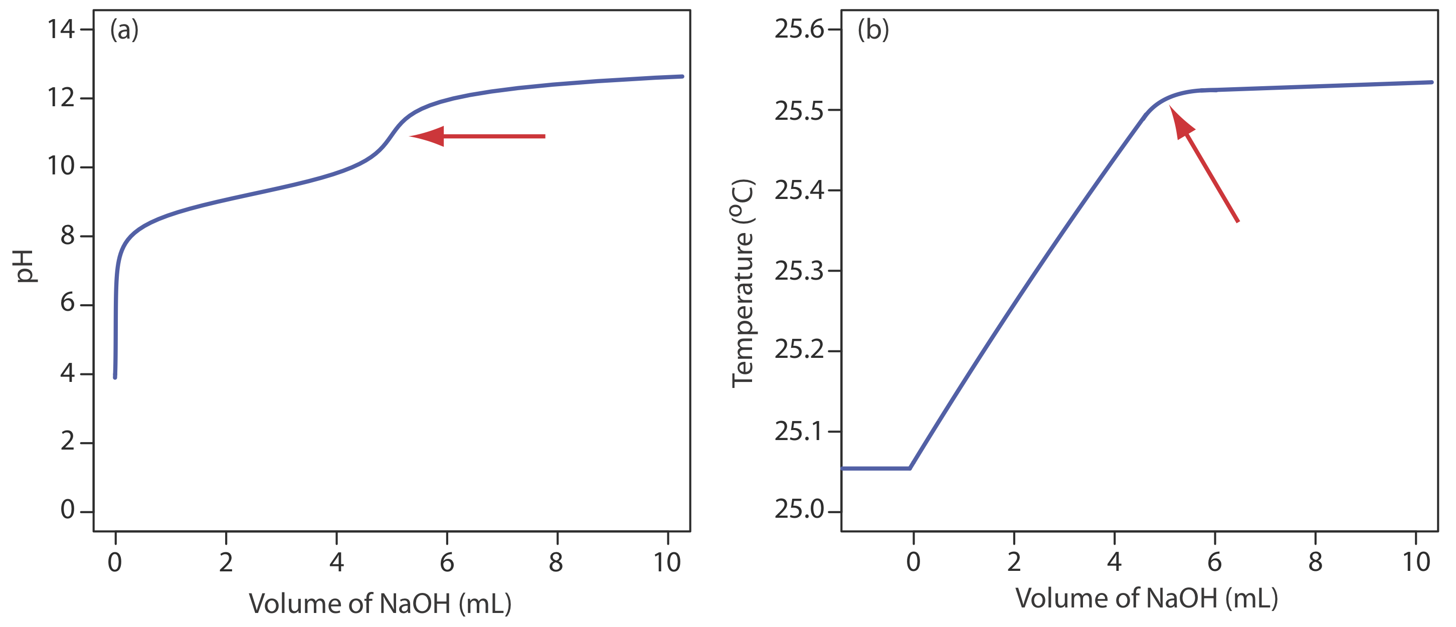
Although not a common method for monitoring an acid–base titration, a thermometric titration has one distinct advantage over the direct or indirect monitoring of pH. As discussed earlier, the use of an indicator or the monitoring of pH is limited by the magnitude of the relevant equilibrium constants. For example, titrating boric acid, H3BO3, with NaOH does not provide a sharp end point when monitoring pH because boric acid’s Ka of \(5.8 \times 10^{-10}\) is too small (Figure \(\PageIndex{11}\)a). Because boric acid’s enthalpy of neutralization is fairly large, –42.7 kJ/mole, its thermometric titration curve provides a useful endpoint (Figure \(\PageIndex{11}\)b).
Titrations in Nonaqueous Solvents
Thus far we have assumed that the titrant and the titrand are aqueous solutions. Although water is the most common solvent for acid–base titrimetry, switching to a nonaqueous solvent can improve a titration’s feasibility.
For an amphoteric solvent, SH, the autoprotolysis constant, Ks, relates the concentration of its protonated form, \(\text{SH}_2^+\), to its deprotonated form, S–
\[\begin{aligned} 2 \mathrm{SH} &\rightleftharpoons\mathrm{SH}_{2}^{+}+\mathrm{S}^{-} \\ K_{\mathrm{s}} &=\left[\mathrm{SH}_{2}^{+}\right][\mathrm{S}^-] \end{aligned} \nonumber\]
and the solvent’s pH and pOH are
\[\begin{array}{l}{\mathrm{pH}=-\log \left[\mathrm{SH}_{2}^{+}\right]} \\ {\mathrm{pOH}=-\log \left[\mathrm{S}^{-}\right]}\end{array} \nonumber\]
You should recognize that Kw is just specific form of Ks when the solvent is water.
The most important limitation imposed by Ks is the change in pH during a titration. To understand why this is true, let’s consider the titration of 50.0 mL of \(1.0 \times 10^{-4}\) M HCl using \(1.0 \times 10^{-4}\) M NaOH as the titrant. Before the equivalence point, the pH is determined by the untitrated strong acid. For example, when the volume of NaOH is 90% of Veq, the concentration of H3O+ is
\[\left[\mathrm{H}_{3} \mathrm{O}^{+}\right]=\frac{M_{a} V_{a}-M_{b} V_{b}}{V_{a}+V_{b}} = \frac{\left(1.0 \times 10^{-4} \ \mathrm{M}\right)(50.0 \ \mathrm{mL})-\left(1.0 \times 10^{-4} \ \mathrm{M}\right)(45.0 \ \mathrm{mL})}{50.0 \ \mathrm{mL}+45.0 \ \mathrm{mL}} = 5.3 \times 10^{-6} \ \mathrm{M} \nonumber\]
and the pH is 5.3. When the volume of NaOH is 110% of Veq, the concentration of OH– is
\[\left[\mathrm{OH}^{-}\right]=\frac{M_{b} V_{b}-M_{a} V_{a}}{V_{a}+V_{b}} = \frac{\left(1.0 \times 10^{-4} \ \mathrm{M}\right)(55.0 \ \mathrm{mL})-\left(1.0 \times 10^{-4} \ \mathrm{M}\right)(50.0 \ \mathrm{mL})}{55.0 \ \mathrm{mL}+50.0 \ \mathrm{mL}} = 4.8 \times 10^{-6} \ \mathrm{M} \nonumber\]
and the pOH is 5.3. The titrand’s pH is
\[\mathrm{pH}=\mathrm{p} K_{w}-\mathrm{pOH}=14.0-5.3=8.7 \nonumber\]
and the change in the titrand’s pH as the titration goes from 90% to 110% of Veq is
\[\Delta \mathrm{pH}=8.7-5.3=3.4 \nonumber\]
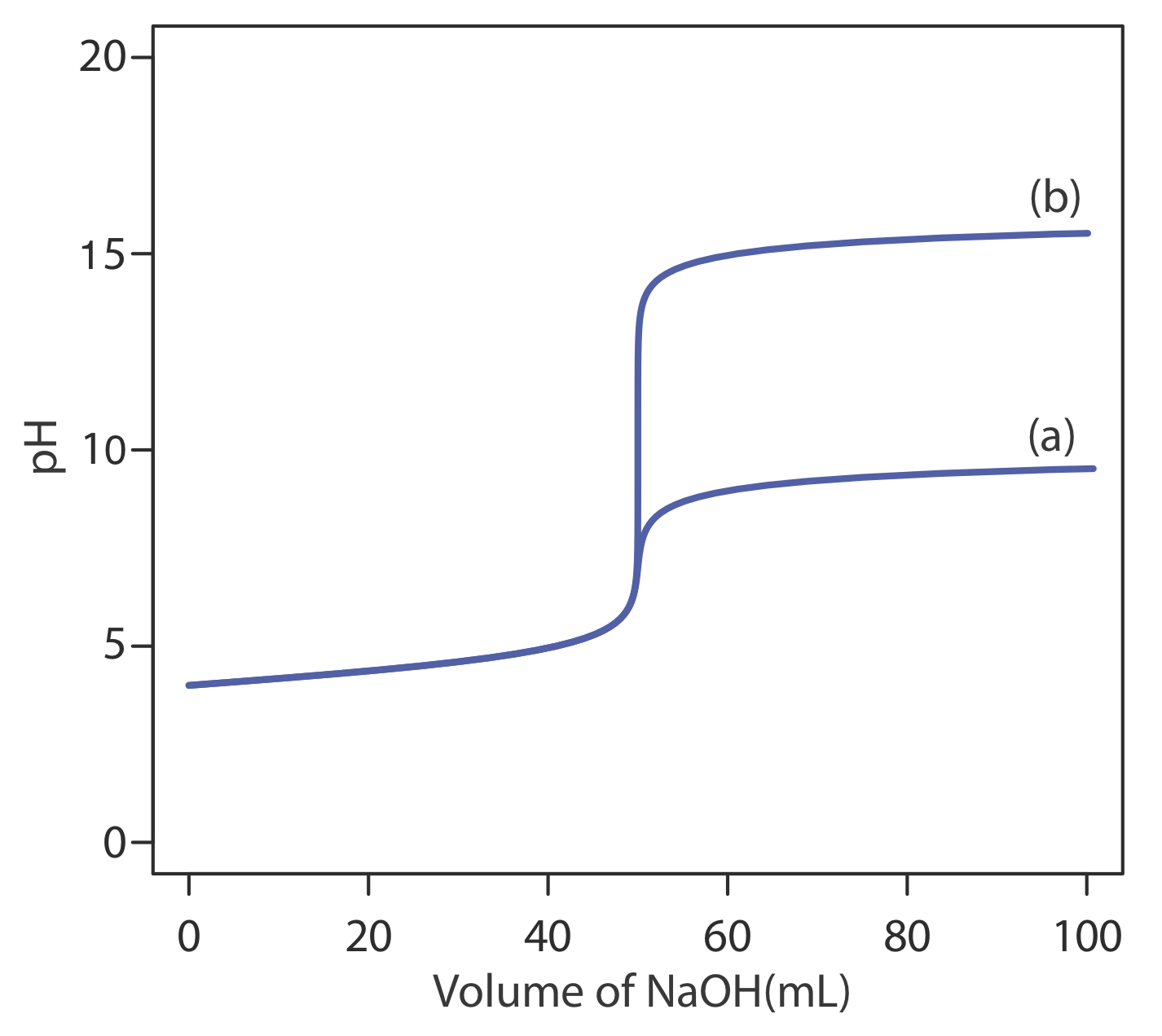
If we carry out the same titration in a nonaqueous amphiprotic solvent that has a Ks of \(1.0 \times 10^{-20}\), the pH after adding 45.0 mL of NaOH is still 5.3. However, the pH after adding 55.0 mL of NaOH is
\[\mathrm{pH}=\mathrm{p} K_{s}-\mathrm{pOH}=20.0-5.3=14.7 \nonumber\]
In this case the change in pH
\[\Delta \mathrm{pH}=14.7-5.3=9.4 \nonumber\]
is significantly greater than that obtained when the titration is carried out in water. Figure \(\PageIndex{12}\) shows the titration curves in both the aqueous and the nonaqueous solvents.
Another parameter that affects the feasibility of an acid–base titration is the titrand’s dissociation constant. Here, too, the solvent plays an important role. The strength of an acid or a base is a relative measure of how easy it is to transfer a proton from the acid to the solvent or from the solvent to the base. For example, HF, with a Ka of \(6.8 \times 10^{-4}\), is a better proton donor than CH3COOH, for which Ka is \(1.75 \times 10^{-5}\).
The strongest acid that can exist in water is the hydronium ion, H3O+. HCl and HNO3 are strong acids because they are better proton donors than H3O+ and essentially donate all their protons to H2O, leveling their acid strength to that of H3O+. In a different solvent HCl and HNO3 may not behave as strong acids.
If we place acetic acid in water the dissociation reaction
\[\mathrm{CH}_{3} \mathrm{COOH}(a q)+\mathrm{H}_{2} \mathrm{O}( l)\rightleftharpoons\mathrm{H}_{3} \mathrm{O}^{+}(a q)+\mathrm{CH}_{3} \mathrm{COO}^{-}(a q) \nonumber\]
does not proceed to a significant extent because CH3COO– is a stronger base than H2O and H3O+ is a stronger acid than CH3COOH. If we place acetic acid in a solvent that is a stronger base than water, such as ammonia, then the reaction
\[\mathrm{CH}_{3} \mathrm{COOH}+\mathrm{NH}_{3}\rightleftharpoons\mathrm{NH}_{4}^{+}+\mathrm{CH}_{3} \mathrm{COO}^{-} \nonumber\]
proceeds to a greater extent. In fact, both HCl and CH3COOH are strong acids in ammonia.
All other things being equal, the strength of a weak acid increases if we place it in a solvent that is more basic than water, and the strength of a weak base increases if we place it in a solvent that is more acidic than water. In some cases, however, the opposite effect is observed. For example, the pKb for NH3 is 4.75 in water and it is 6.40 in the more acidic glacial acetic acid. In contradiction to our expectations, NH3 is a weaker base in the more acidic solvent. A full description of the solvent’s effect on the pKa of weak acid or the pKb of a weak base is beyond the scope of this text. You should be aware, however, that a titration that is not feasible in water may be feasible in a different solvent.
Representative Method 9.2.1: Determination of Protein in Bread
The best way to appreciate the theoretical and the practical details discussed in this section is to carefully examine a typical acid–base titrimetric method. Although each method is unique, the following description of the determination of protein in bread provides an instructive example of a typical procedure. The description here is based on Method 13.86 as published in Official Methods of Analysis, 8th Ed., Association of Official Agricultural Chemists: Washington, D. C., 1955.
Description of the Methods
This method is based on a determination of %w/w nitrogen using the Kjeldahl method. The protein in a sample of bread is oxidized to \(\text{NH}_4^+\) using hot concentrated H2SO4. After making the solution alkaline, which converts \(\text{NH}_4^+\) to NH3, the ammonia is distilled into a flask that contains a known amount of HCl. The amount of unreacted HCl is determined by a back titration using a standard strong base titrant. Because different cereal proteins contain similar amounts of nitrogen—on average there are 5.7 g protein for every gram of nitrogen—we multiply the experimentally determined %w/w N by a factor of 5.7 gives the %w/w protein in the sample.
Procedure
Transfer a 2.0-g sample of bread, which previously has been air-dried and ground into a powder, to a suitable digestion flask along with 0.7 g of a HgO catalyst, 10 g of K2SO4, and 25 mL of concentrated H2SO4. Bring the solution to a boil. Continue boiling until the solution turns clear and then boil for at least an additional 30 minutes. After cooling the solution below room temperature, remove the Hg2+ catalyst by adding 200 mL of H2O and 25 mL of 4% w/v K2S. Add a few Zn granules to serve as boiling stones and 25 g of NaOH. Quickly connect the flask to a distillation apparatus and distill the NH3 into a collecting flask that contains a known amount of standardized HCl. The tip of the condenser must be placed below the surface of the strong acid. After the distillation is complete, titrate the excess strong acid with a standard solution of NaOH using methyl red as an indicator (Figure \(\PageIndex{13}\)).
Questions
1. Oxidizing the protein converts all of its nitrogen to \(\text{NH}_4^+\). Why is the amount of nitrogen not determined by directly titrating the \(\text{NH}_4^+\) with a strong base?
There are two reasons for not directly titrating the ammonium ion. First, because \(\text{NH}_4^+\) is a very weak acid (its Ka is \(5.6 \times 10^{-10}\)), its titration with NaOH has a poorly-defined end point. Second, even if we can determine the end point with acceptable accuracy and precision, the solution also contains a substantial concentration of unreacted H2SO4. The presence of two acids that differ greatly in concentration makes for a difficult analysis. If the titrant’s concentration is similar to that of H2SO4, then the equivalence point volume for the titration of \(\text{NH}_4^+\) is too small to measure reliably. On the other hand, if the titrant’s concentration is similar to that of \(\text{NH}_4^+\), the volume needed to neutralize the H2SO4 is unreasonably large.
2. Ammonia is a volatile compound as evidenced by the strong smell of even dilute solutions. This volatility is a potential source of determinate error. Is this determinate error negative or positive?
Any loss of NH3 is loss of nitrogen and, therefore, a loss of protein. The result is a negative determinate error.
3. Identify the steps in this procedure that minimize the determinate error from the possible loss of NH3.
Three specific steps minimize the loss of ammonia: (1) the solution is cooled below room temperature before we add NaOH; (2) after we add NaOH, the digestion flask is quickly connected to the distillation apparatus; and (3) we place the condenser’s tip below the surface of the HCl to ensure that the NH3 reacts with the HCl before it is lost through volatilization.
4. How does K2S remove Hg2+, and why is its removal important?
Adding sulfide precipitates Hg2+ as HgS. This is important because NH3 forms stable complexes with many metal ions, including Hg2+. Any NH3 that reacts with Hg2+ is not collected during distillation, providing another source of determinate error.
Quantitative Applications
Although many quantitative applications of acid–base titrimetry have been replaced by other analytical methods, a few important applications continue to find use. In this section we review the general application of acid–base titrimetry to the analysis of inorganic and organic compounds, with an emphasis on applications in environmental and clinical analysis. First, however, we discuss the selection and standardization of acidic and basic titrants.
Selecting and Standardizing a Titrant
The most common strong acid titrants are HCl, HClO4, and H2SO4. Solutions of these titrants usually are prepared by diluting a commercially available concentrated stock solution. Because the concentration of a concentrated acid is known only approximately, the titrant’s concentration is determined by standardizing against one of the primary standard weak bases listed in Table \(\PageIndex{4}\).
The nominal concentrations of the concentrated stock solutions are 12.1 M HCl, 11.7 M HClO4, and 18.0 M H2SO4. The actual concentrations of these acids are given as %w/v and vary slightly from lot-to-lot.
The most common strong base titrant is NaOH, which is available both as an impure solid and as an approximately 50% w/v solution. Solutions of NaOH are standardized against any of the primary weak acid standards listed in Table \(\PageIndex[4|\).
Using NaOH as a titrant is complicated by potential contamination from the following reaction between dissolved CO2 and OH–.
\[\mathrm{CO}_{2}(a q)+2 \mathrm{OH}^{-}(a q) \rightarrow \mathrm{CO}_{3}^{2-}(a q)+\mathrm{H}_{2} \mathrm{O}( l) \label{9.7}\]
Any solution in contact with the atmosphere contains a small amount of CO2(aq) from the equilibrium
\[\mathrm{CO}_{2}(g)\rightleftharpoons\mathrm{CO}_{2}(a q) \nonumber\]
During the titration, NaOH reacts both with the titrand and with CO2, which increases the volume of NaOH needed to reach the titration’s end point. This is not a problem if the end point pH is less than 6. Below this pH the \(\text{CO}_3^{2-}\) from reaction \ref{9.7} reacts with H3O+ to form carbonic acid.
\[\mathrm{CO}_{3}^{2-}(a q)+2 \mathrm{H}_{3} \mathrm{O}^{+}(a q) \rightarrow 2 \mathrm{H}_{2} \mathrm{O}(l)+\mathrm{H}_{2} \mathrm{CO}_{3}(a q). \label{9.8}\]
Combining reaction \ref{9.7} and reaction \ref{9.8} gives an overall reaction that does not include OH–.
\[\mathrm{CO}_{2}(a q)+\mathrm{H}_{2} \mathrm{O}(l ) \longrightarrow \mathrm{H}_{2} \mathrm{CO}_{3}(a q) \nonumber\]
Under these conditions the presence of CO2 does not affect the quantity of OH– used in the titration and is not a source of determinate error.
If the end point pH is between 6 and 10, however, the neutralization of \(\text{CO}_3^{2-}\) requires one proton
\[\mathrm{CO}_{3}^{2-}(a q)+\mathrm{H}_{3} \mathrm{O}^{+}(a q) \rightarrow \mathrm{H}_{2} \mathrm{O}(l)+\mathrm{HCO}_{3}^{-}(a q) \nonumber\]
and the net reaction between CO2 and OH– is
\[\mathrm{CO}_{2}(a q)+\mathrm{OH}^{-}(a q) \rightarrow \mathrm{HCO}_{3}^{-}(a q) \nonumber\]
Under these conditions some OH– is consumed in neutralizing CO2, which results in a determinate error. We can avoid the determinate error if we use the same end point pH for both the standardization of NaOH and the analysis of our analyte, although this is not always practical.
Solid NaOH is always contaminated with carbonate due to its contact with the atmosphere, and we cannot use it to prepare a carbonate-free solution of NaOH. Solutions of carbonate-free NaOH are prepared from 50% w/v NaOH because Na2CO3 is insoluble in concentrated NaOH. When CO2 is absorbed, Na2CO3 precipitates and settles to the bottom of the container, which allow access to the carbonate-free NaOH. When pre- paring a solution of NaOH, be sure to use water that is free from dissolved CO2. Briefly boiling the water expels CO2; after it cools, the water is used to prepare carbonate-free solutions of NaOH. A solution of carbonate-free NaOH is relatively stable if we limit its contact with the atmosphere. Standard solutions of sodium hydroxide are not stored in glass bottles as NaOH reacts with glass to form silicate; instead, store such solutions in polyethylene bottles.
Inorganic Analysis
Acid–base titrimetry is a standard method for the quantitative analysis of many inorganic acids and bases. A standard solution of NaOH is used to determine the concentration of inorganic acids, such as H3PO4 or H3AsO4, and inorganic bases, such as Na2CO3 are analyzed using a standard solution of HCl.
If an inorganic acid or base that is too weak to be analyzed by an aqueous acid–base titration, it may be possible to complete the analysis by adjusting the solvent or by an indirect analysis. For example, when analyzing boric acid, H3BO3, by titrating with NaOH, accuracy is limited by boric acid’s small acid dissociation constant of \(5.8 \times 10^{-10}\). Boric acid’s Ka value increases to \(1.5 \times 10^{-4}\) in the presence of mannitol, because it forms a stable complex with the borate ion, which results is a sharper end point and a more accurate titration. Similarly, the analysis of ammonium salts is limited by the ammonium ion’ small acid dissociation constant of \(5.7 \times 10^{-10}\). We can determine \(\text{NH}_4^+\) indirectly by using a strong base to convert it to NH3, which is removed by distillation and titrated with HCl. Because NH3 is a stronger weak base than \(\text{NH}_4^+\) is a weak acid (its Kb is \(1.58 \times 10^{-5}\)), the titration has a sharper end point.
We can analyze a neutral inorganic analyte if we can first convert it into an acid or a base. For example, we can determine the concentration of \(\text{NO}_3^-\) by reducing it to NH3 in a strongly alkaline solution using Devarda’s alloy, a mixture of 50% w/w Cu, 45% w/w Al, and 5% w/w Zn.
\[3 \mathrm{NO}_{3}^{-}(a q)+8 \mathrm{Al}(s)+5 \mathrm{OH}^{-}(a q)+2 \mathrm{H}_{2} \mathrm{O}(l) \rightarrow 8 \mathrm{AlO}_{2}^{-}(a q)+3 \mathrm{NH}_{3}(a q) \nonumber\]
The NH3 is removed by distillation and titrated with HCl. Alternatively, we can titrate \(\text{NO}_3^-\) as a weak base by placing it in an acidic nonaqueous solvent, such as anhydrous acetic acid, and using HClO4 as a titrant.
Acid–base titrimetry continues to be listed as a standard method for the determination of alkalinity, acidity, and free CO2 in waters and wastewaters. Alkalinity is a measure of a sample’s capacity to neutralize acids. The most important sources of alkalinity are OH–, \(\text{HCO}_3^-\), and \(\text{CO}_3^{2-}\), although other weak bases, such as phosphate, may contribute to the overall alkalinity. Total alkalinity is determined by titrating to a fixed end point pH of 4.5 (or to the bromocresol green end point) using a standard solution of HCl or H2SO4. Results are reported as mg CaCO3/L.
Although a variety of strong bases and weak bases may contribute to a sample’s alkalinity, a single titration cannot distinguish between the possible sources. Reporting the total alkalinity as if CaCO3 is the only source provides a means for comparing the acid-neutralizing capacities of different samples.
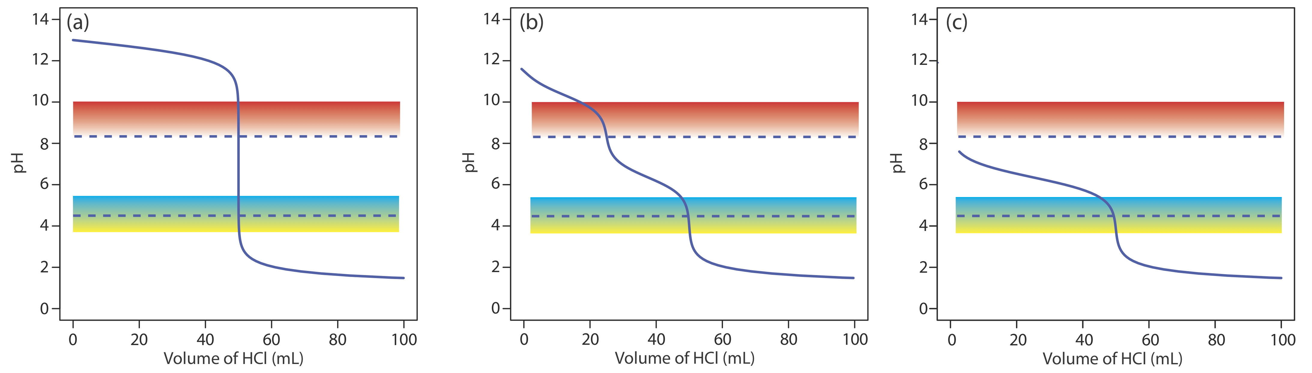
When the sources of alkalinity are limited to OH–, \(\text{HCO}_3^-\), and \(\text{CO}_3^{2-}\), separate titrations to a pH of 4.5 (or the bromocresol green end point) and a pH of 8.3 (or the phenolphthalein end point) allow us to determine which species are present and their respective concentrations. Titration curves for OH–, \(\text{HCO}_3^-\), and \(\text{CO}_3^{2-}\)are shown in Figure \(\PageIndex{14}\). For a solution that contains OH– alkalinity only, the volume of strong acid needed to reach each of the two end points is identical (Figure \(\PageIndex{14}\)a). When the only source of alkalinity is \(\text{CO}_3^{2-}\), the volume of strong acid needed to reach the end point at a pH of 4.5 is exactly twice that needed to reach the end point at a pH of 8.3 (Figure \(\PageIndex{14}\)b). If a solution contains \(\text{HCO}_3^-\) alkalinity only, the volume of strong acid needed to reach the end point at a pH of 8.3 is zero, but that for the pH 4.5 end point is greater than zero (Figure \(\PageIndex{14}\)c).
A mixture of OH– and \(\text{CO}_3^{2-}\) or a mixture of \(\text{HCO}_3^-\) and \(\text{CO}_3^{2-}\) also is possible. Consider, for example, a mixture of OH– and \(\text{CO}_3^{2-}\). The volume of strong acid to titrate OH– is the same whether we titrate to a pH of 8.3 or a pH of 4.5. Titrating \(\text{CO}_3^{2-}\) to a pH of 4.5, however, requires twice as much strong acid as titrating to a pH of 8.3. Consequently, when we titrate a mixture of these two ions, the volume of strong acid needed to reach a pH of 4.5 is less than twice that needed to reach a pH of 8.3. For a mixture of \(\text{HCO}_3^-\) and \(\text{CO}_3^{2-}\) the volume of strong acid needed to reach a pH of 4.5 is more than twice that needed to reach a pH of 8.3. Table \(\PageIndex{5}\) summarizes the relationship between the sources of alkalinity and the volumes of titrant needed to reach the two end points.
A mixture of OH– and \(\text{HCO}_3^-\) is unstable with respect to the formation of \(\text{CO}_3^{2-}\). Problem 15 in the end-of-chapter problems asks you to explain why this is true.
Acidity is a measure of a water sample’s capacity to neutralize base and is divided into strong acid and weak acid acidity. Strong acid acidity from inorganic acids such as HCl, HNO3, and H2SO4 is common in industrial effluents and in acid mine drainage. Weak acid acidity usually is dominated by the formation of H2CO3 from dissolved CO2, but also includes contributions from hydrolyzable metal ions such as Fe3+, Al3+, and Mn2+. In addition, weak acid acidity may include a contribution from organic acids.
Acidity is determined by titrating with a standard solution of NaOH to a fixed pH of 3.7 (or the bromothymol blue end point) and to a fixed pH of 8.3 (or the phenolphthalein end point). Titrating to a pH of 3.7 provides a measure of strong acid acidity, and titrating to a pH of 8.3 provides a measure of total acidity. Weak acid acidity is the difference between the total acidity and the strong acid acidity. Results are expressed as the amount of CaCO3 that can be neutralized by the sample’s acidity. An alternative approach for determining strong acid and weak acid acidity is to obtain a potentiometric titration curve and use a Gran plot to determine the two equivalence points. This approach has been used, for example, to determine the forms of acidity in atmospheric aerosols [Ferek, R. J.; Lazrus, A. L.; Haagenson, P. L.; Winchester, J. W. Environ. Sci. Technol. 1983, 17, 315–324].
As is the case with alkalinity, acidity is reported as mg CaCO3/L.
Water in contact with either the atmosphere or with carbonate-bearing sediments contains free CO2 in equilibrium with CO2(g) and with aqueous H2CO3, \(\text{HCO}_3^-\) and \(\text{CO}_3^{2-}\). The concentration of free CO2 is determined by titrating with a standard solution of NaOH to the phenolphthalein end point, or to a pH of 8.3, with results reported as mg CO2/L. This analysis essentially is the same as that for the determination of total acidity and is used only for water samples that do not contain strong acid acidity.
Free CO2 is the same thing as CO2(aq).
Organic Analysis
Acid–base titrimetry continues to have a small, but important role for the analysis of organic compounds in pharmaceutical, biochemical, agricultur- al, and environmental laboratories. Perhaps the most widely employed acid–base titration is the Kjeldahl analysis for organic nitrogen. Examples of analytes determined by a Kjeldahl analysis include caffeine and saccharin in pharmaceutical products, proteins in foods, and the analysis of nitrogen in fertilizers, sludges, and sediments. Any nitrogen present in a –3 oxidation state is oxidized quantitatively to \(\text{NH}_4^+\). Because some aromatic heterocyclic compounds, such as pyridine, are difficult to oxidize, a catalyst is used to ensure a quantitative oxidation. Nitrogen in other oxidation states, such as nitro and azo nitrogens, are oxidized to N2, which results in a negative determinate error. Including a reducing agent, such as salicylic acid, converts this nitrogen to a –3 oxidation state, eliminating this source of error. Table \(\PageIndex{6}\) provides additional examples in which an element is converted quantitatively into a titratable acid or base.
Several organic functional groups are weak acids or weak bases. Carboxylic (–COOH), sulfonic (–SO3H) and phenolic (–C6H5OH) functional groups are weak acids that are titrated successfully in either aqueous or non-aqueous solvents. Sodium hydroxide is the titrant of choice for aqueous solutions. Nonaqueous titrations often are carried out in a basic solvent, such as ethylenediamine, using tetrabutylammonium hydroxide, (C4H9)4NOH, as the titrant. Aliphatic and aromatic amines are weak bases that are titrated using HCl in aqueous solutions, or HClO4 in glacial acetic acid. Other functional groups are analyzed indirectly following a reaction that produces or consumes an acid or base. Typical examples are shown in Table \(\PageIndex{7}\).
Many pharmaceutical compounds are weak acids or weak bases that are analyzed by an aqueous or a nonaqueous acid–base titration; examples include salicylic acid, phenobarbital, caffeine, and sulfanilamide. Amino acids and proteins are analyzed in glacial acetic acid using HClO4 as the titrant. For example, a procedure for determining the amount of nutritionally available protein uses an acid–base titration of lysine residues [(a) Molnár-Perl, I.; Pintée-Szakács, M. Anal. Chim. Acta 1987, 202, 159–166; (b) Barbosa, J.; Bosch, E.; Cortina, J. L.; Rosés, M. Anal. Chim. Acta 1992, 256, 177–181].
Quantitative Calculations
The quantitative relationship between the titrand and the titrant is determined by the titration reaction’s stoichiometry. If the titrand is polyprotic, then we must know to which equivalence point we are titrating. The following example illustrates how we can use a ladder diagram to determine a titration reaction’s stoichiometry.
A 50.00-mL sample of a citrus drink requires 17.62 mL of 0.04166 M NaOH to reach the phenolphthalein end point. Express the sample’s acidity as grams of citric acid, C6H8O7, per 100 mL.
Solution
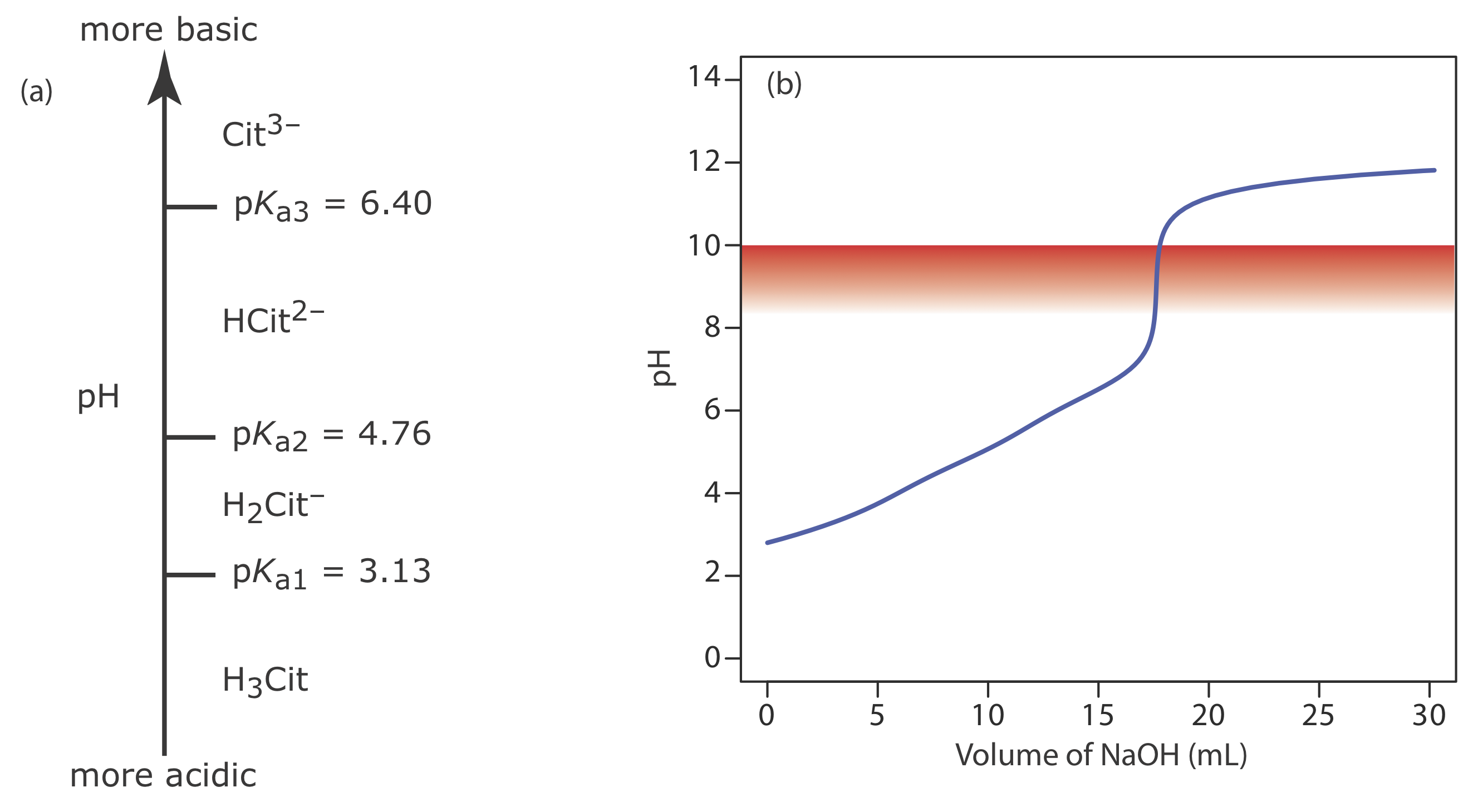
Because citric acid is a triprotic weak acid, we first must determine if the phenolphthalein end point corresponds to the first, second, or third equivalence point. Citric acid’s ladder diagram is shown in Figure \(\PageIndex{15}\)a. Based on this ladder diagram, the first equivalence point is between a pH of 3.13 and a pH of 4.76, the second equivalence point is between a pH of 4.76 and a pH of 6.40, and the third equivalence point is greater than a pH of 6.40. Because phenolphthalein’s end point pH is 8.3–10.0 (see Table \(\PageIndex{3}\)), the titration must proceed to the third equivalence point and the titration reaction is
\[ \mathrm{C}_{6} \mathrm{H}_{8} \mathrm{O}_{7}(a q)+3 \mathrm{OH}^{-}(a q) \longrightarrow \mathrm{C}_{6} \mathrm{H}_{5} \mathrm{O}_{7}^{3-}(a q)+3 \mathrm{H}_{2} \mathrm{O}(l) \nonumber\]
To reach the equivalence point, each mole of citric acid consumes three moles of NaOH; thus
\[(0.04166 \ \mathrm{M} \ \mathrm{NaOH})(0.01762 \ \mathrm{L} \ \mathrm{NaOH})=7.3405 \times 10^{-4} \ \mathrm{mol} \ \mathrm{NaOH} \nonumber\]
\[7.3405 \times 10^{-4} \ \mathrm{mol} \ \mathrm{NaOH} \times \frac{1 \ \mathrm{mol} \ \mathrm{C}_{6} \mathrm{H}_{8} \mathrm{O}_{7}}{3 \ \mathrm{mol} \ \mathrm{NaOH}}= 2.4468 \times 10^{-4} \ \mathrm{mol} \ \mathrm{C}_{6} \mathrm{H}_{8} \mathrm{O}_{7} \nonumber\]
\[2.4468 \times 10^{-4} \ \mathrm{mol} \ \mathrm{C}_{6} \mathrm{H}_{8} \mathrm{O}_{7} \times \frac{192.1 \ \mathrm{g} \ \mathrm{C}_{6} \mathrm{H}_{8} \mathrm{O}_{7}}{\mathrm{mol} \ \mathrm{C}_{6} \mathrm{H}_{8} \mathrm{O}_{7}}=0.04700 \ \mathrm{g} \ \mathrm{C}_{6} \mathrm{H}_{8} \mathrm{O}_{7} \nonumber\]
Because this is the amount of citric acid in a 50.00 mL sample, the concentration of citric acid in the citrus drink is 0.09400 g/100 mL. The complete titration curve is shown in Figure \(\PageIndex{15}\)b.
Your company recently received a shipment of salicylic acid, C7H6O3, for use in the production of acetylsalicylic acid (aspirin). You can accept the shipment only if the salicylic acid is more than 99% pure. To evaluate the shipment’s purity, you dissolve a 0.4208-g sample in water and titrate to the phenolphthalein end point, using 21.92 mL of 0.1354 M NaOH. Report the shipment’s purity as %w/w C7H6O3. Salicylic acid is a diprotic weak acid with pKa values of 2.97 and 13.74.
- Answer
-
Because salicylic acid is a diprotic weak acid, we must first determine to which equivalence point it is being titrated. Using salicylic acid’s pKa values as a guide, the pH at the first equivalence point is between 2.97 and 13.74, and the second equivalence points is at a pH greater than 13.74. From Table \(\PageIndex{3}\), phenolphthalein’s end point is in the pH range 8.3–10.0. The titration, therefore, is to the first equivalence point for which the moles of NaOH equal the moles of salicylic acid; thus
\[(0.1354 \ \mathrm{M})(0.02192 \ \mathrm{L})=2.968 \times 10^{-3} \ \mathrm{mol} \ \mathrm{NaOH} \nonumber\]
\[2.968 \times 10^{-3} \ \mathrm{mol} \ \mathrm{NaOH} \times \frac{1 \ \mathrm{mol} \ \mathrm{C}_{7} \mathrm{H}_{6} \mathrm{O}_{3}}{\mathrm{mol} \ \mathrm{NaOH}} \times \frac{138.12 \ \mathrm{g} \ \mathrm{C}_{7} \mathrm{H}_{6} \mathrm{O}_{3}}{\mathrm{mol} \ \mathrm{C}_{7} \mathrm{H}_{6} \mathrm{O}_{3}}=0.4099 \ \mathrm{g} \ \mathrm{C}_{7} \mathrm{H}_{6} \mathrm{O}_{3} \nonumber\]
\[\frac{0.4099 \ \mathrm{g} \ \mathrm{C}_{7} \mathrm{H}_{6} \mathrm{O}_{3}}{0.4208 \ \mathrm{g} \text { sample }} \times 100=97.41 \ \% \mathrm{w} / \mathrm{w} \ \mathrm{C}_{7} \mathrm{H}_{6} \mathrm{O}_{3} \nonumber\]
Because the purity of the sample is less than 99%, we reject the shipment.
In an indirect analysis the analyte participates in one or more preliminary reactions, one of which produces or consumes acid or base. Despite the additional complexity, the calculations are straightforward.
The purity of a pharmaceutical preparation of sulfanilamide, C6H4N2O2S, is determined by oxidizing the sulfur to SO2 and bubbling it through H2O2 to produce H2SO4. The acid is titrated to the bromothymol blue end point using a standard solution of NaOH. Calculate the purity of the preparation given that a 0.5136-g sample requires 48.13 mL of 0.1251 M NaOH.
Solution
The bromothymol blue end point has a pH range of 6.0–7.6. Sulfuric acid is a diprotic acid, with a pKa2 of 1.99 (the first Ka value is very large and the acid dissociation reaction goes to completion, which is why H2SO4 is a strong acid). The titration, therefore, proceeds to the second equivalence point and the titration reaction is
\[\mathrm{H}_{2} \mathrm{SO}_{4}(a q)+2 \mathrm{OH}^{-}(a q) \longrightarrow 2 \mathrm{H}_{2} \mathrm{O}(l)+\mathrm{SO}_{4}^{2-}(a q) \nonumber\]
Using the titration results, there are
\[(0.1251 \ \mathrm{M} \ \mathrm{NaOH})(0.04813 \ \mathrm{L} \ \mathrm{NaOH})=6.021 \times 10^{-3} \ \mathrm{mol} \ \mathrm{NaOH} \nonumber\]
\[6.012 \times 10^{-3} \text{ mol NaOH} \times \frac{1 \text{ mol} \mathrm{H}_{2} \mathrm{SO}_{4}} {2 \text{ mol NaOH}} = 3.010 \times 10^{-3} \text{ mol} \mathrm{H}_{2} \mathrm{SO}_{4} \nonumber\]
\[3.010 \times 10^{-3} \ \mathrm{mol} \ \mathrm{H}_{2} \mathrm{SO}_{4} \times \frac{1 \ \mathrm{mol} \text{ S}}{\mathrm{mol} \ \mathrm{H}_{2} \mathrm{SO}_{4}} \times \ \frac{1 \ \mathrm{mol} \ \mathrm{C}_{6} \mathrm{H}_{4} \mathrm{N}_{2} \mathrm{O}_{2} \mathrm{S}}{\mathrm{mol} \text{ S}} \times \frac{168.17 \ \mathrm{g} \ \mathrm{C}_{6} \mathrm{H}_{4} \mathrm{N}_{2} \mathrm{O}_{2} \mathrm{S}}{\mathrm{mol} \ \mathrm{C}_{6} \mathrm{H}_{4} \mathrm{N}_{2} \mathrm{O}_{2} \mathrm{S}}= 0.5062 \ \mathrm{g} \ \mathrm{C}_{6} \mathrm{H}_{4} \mathrm{N}_{2} \mathrm{O}_{2} \mathrm{S} \nonumber\]
produced when the SO2 is bubbled through H2O2. Because all the sulfur in H2SO4 comes from the sulfanilamide, we can use a conservation of mass to determine the amount of sulfanilamide in the sample.
\[\frac{0.5062 \ \mathrm{g} \ \mathrm{C}_{6} \mathrm{H}_{4} \mathrm{N}_{2} \mathrm{O}_{2} \mathrm{S}}{0.5136 \ \mathrm{g} \text { sample }} \times 100=98.56 \ \% \mathrm{w} / \mathrm{w} \ \mathrm{C}_{6} \mathrm{H}_{4} \mathrm{N}_{2} \mathrm{O}_{2} \mathrm{S} \nonumber\]
The concentration of NO2 in air is determined by passing the sample through a solution of H2O2, which oxidizes NO2 to HNO3, and titrating the HNO3 with NaOH. What is the concentration of NO2, in mg/L, if a 5.0 L sample of air requires 9.14 mL of 0.01012 M NaOH to reach the methyl red end point
- Answer
-
The moles of HNO3 produced by pulling the sample through H2O2 is
\[(0.01012 \ \mathrm{M})(0.00914 \ \mathrm{L}) \times \frac{1 \ \mathrm{mol} \ \mathrm{HNO}_{3}}{\mathrm{mol} \ \mathrm{NaOH}}=9.25 \times 10^{-5} \ \mathrm{mol} \ \mathrm{HNO}_{3} \nonumber\]
A conservation of mass on nitrogen requires that each mole of NO2 produces one mole of HNO3; thus, the mass of NO2 in the sample is
\[9.25 \times 10^{-5} \ \mathrm{mol} \ \mathrm{HNO}_{3} \times \frac{1 \ \mathrm{mol} \ \mathrm{NO}_{2}}{\mathrm{mol} \ \mathrm{HNO}_{3}} \times \frac{46.01 \ \mathrm{g} \ \mathrm{NO}_{2}}{\mathrm{mol} \ \mathrm{NO}_{2}}=4.26 \times 10^{-3} \ \mathrm{g} \ \mathrm{NO}_{2} \nonumber\]
and the concentration of NO2 is
\[\frac{4.26 \times 10^{-3} \ \mathrm{g} \ \mathrm{NO}_{2}}{5 \ \mathrm{L} \text { air }} \times \frac{1000 \ \mathrm{mg}}{\mathrm{g}}=0.852 \ \mathrm{mg} \ \mathrm{NO}_{2} \ \mathrm{L} \text { air } \nonumber\]
For a back titration we must consider two acid–base reactions. Again, the calculations are straightforward.
The amount of protein in a sample of cheese is determined by a Kjeldahl analysis for nitrogen. After digesting a 0.9814-g sample of cheese, the nitrogen is oxidized to \(\text{NH}_4^+\), converted to NH3 with NaOH, and the NH3 distilled into a collection flask that contains 50.00 mL of 0.1047 M HCl. The excess HCl is back titrated with 0.1183 M NaOH, requiring 22.84 mL to reach the bromothymol blue end point. Report the %w/w protein in the cheese assuming there are 6.38 grams of protein for every gram of nitrogen in most dairy products.
Solution
The HCl in the collection flask reacts with two bases
\[\mathrm{HCl}(a q)+\mathrm{NH}_{3}(a q) \rightarrow \mathrm{NH}_{4}^{+}(a q)+\mathrm{Cl}^{-}(a q) \nonumber\]
\[\mathrm{HCl}(a q)+\mathrm{OH}^{-}(a q) \rightarrow \mathrm{H}_{2} \mathrm{O}(l)+\mathrm{Cl}^{-}(a q) \nonumber\]
The collection flask originally contains
\[(0.1047 \ \mathrm{M \ HCl})(0.05000 \ \mathrm{L \ HCl})=5.235 \times 10^{-3} \mathrm{mol} \ \mathrm{HCl} \nonumber\]
of which
\[(0.1183 \ \mathrm{M} \ \mathrm{NaOH})(0.02284 \ \mathrm{L} \ \mathrm{NaOH}) \times \frac{1 \ \mathrm{mol} \ \mathrm{HCl}}{\mathrm{mol} \ \mathrm{NaOH}}=2.702 \times 10^{-3} \ \mathrm{mol} \ \mathrm{HCl} \nonumber\]
react with NaOH. The difference between the total moles of HCl and the moles of HCl that react with NaOH is the moles of HCl that react with NH3.
\[5.235 \times 10^{-3} \ \mathrm{mol} \ \mathrm{HCl}-2.702 \times 10^{-3} \ \mathrm{mol} \ \mathrm{HCl} =2.533 \times 10^{-3} \ \mathrm{mol} \ \mathrm{HCl} \nonumber\]
Because all the nitrogen in NH3 comes from the sample of cheese, we use a conservation of mass to determine the grams of nitrogen in the sample.
\[2.533 \times 10^{-3} \ \mathrm{mol} \ \mathrm{HCl} \times \frac{1 \ \mathrm{mol} \ \mathrm{NH}_{3}}{\mathrm{mol} \ \mathrm{HCl}} \times \frac{14.01 \ \mathrm{g} \ \mathrm{N}}{\mathrm{mol} \ \mathrm{NH}_{3}}=0.03549 \ \mathrm{g} \ \mathrm{N} \nonumber\]
The mass of protein, therefore, is
\[0.03549 \ \mathrm{g} \ \mathrm{N} \times \frac{6.38 \ \mathrm{g} \text { protein }}{\mathrm{g} \ \mathrm{N}}=0.2264 \ \mathrm{g} \text { protein } \nonumber\]
and the % w/w protein is
\[\frac{0.2264 \ \mathrm{g} \text { protein }}{0.9814 \ \mathrm{g} \text { sample }} \times 100=23.1 \ \% \mathrm{w} / \mathrm{w} \text { protein } \nonumber\]
Limestone consists mainly of CaCO3, with traces of iron oxides and other metal oxides. To determine the purity of a limestone, a 0.5413-g sample is dissolved using 10.00 mL of 1.396 M HCl. After heating to expel CO2, the excess HCl was titrated to the phenolphthalein end point, requiring 39.96 mL of 0.1004 M NaOH. Report the sample’s purity as %w/w CaCO3.
- Answer
-
The total moles of HCl used in this analysis is
\[(1.396 \ \mathrm{M})(0.01000 \ \mathrm{L})=1.396 \times 10^{-2} \ \mathrm{mol} \ \mathrm{HCl} \nonumber\]
Of the total moles of HCl
\[(0.1004 \ \mathrm{M} \ \mathrm{NaOH})(0.03996 \ \mathrm{L}) \times \frac{1 \ \mathrm{mol} \ \mathrm{HCl}}{\mathrm{mol} \ \mathrm{NaOH}} =4.012 \times 10^{-3} \ \mathrm{mol} \ \mathrm{HCl} \nonumber\]
are consumed in the back titration with NaOH, which means that
\[ 1.396 \times 10^{-2} \ \mathrm{mol} \ \mathrm{HCl}-4.012 \times 10^{-3} \ \mathrm{mol} \ \mathrm{HCl} \\ =9.95 \times 10^{-3} \ \mathrm{mol} \ \mathrm{HCl} \nonumber\]
react with the CaCO3. Because \(\text{CO}_3^{2-}\) is dibasic, each mole of CaCO3 consumes two moles of HCl; thus
\[9.95 \times 10^{-3} \ \mathrm{mol} \ \mathrm{HCl} \times \frac{1 \ \mathrm{mol} \ \mathrm{CaCO}_{3}}{2 \ \mathrm{mol} \ \mathrm{HCl}} \times \\ \frac{100.09 \ \mathrm{g} \ \mathrm{CaCO}_{3}}{\mathrm{mol} \ \mathrm{CaCO}_{3}}=0.498 \ \mathrm{g} \ \mathrm{CaCO}_{3} \nonumber\]
\[\frac{0.498 \ \mathrm{g} \ \mathrm{CaCO}_{3}}{0.5143 \ \mathrm{g} \text { sample }} \times 100=96.8 \ \% \mathrm{w} / \mathrm{w} \ \mathrm{CaCO}_{3} \nonumber\]
Earlier we noted that we can use an acid–base titration to analyze a mixture of acids or bases by titrating to more than one equivalence point. The concentration of each analyte is determined by accounting for its contribution to each equivalence point.
The alkalinity of natural waters usually is controlled by OH–, \(\text{HCO}_3^-\), and \(\text{CO}_3^{2-}\), present singularly or in combination. Titrating a 100.0-mL sample to a pH of 8.3 requires 18.67 mL of 0.02812 M HCl. A second 100.0-mL aliquot requires 48.12 mL of the same titrant to reach a pH of 4.5. Identify the sources of alkalinity and their concentrations in milligrams per liter.
Solution
Because the volume of titrant to reach a pH of 4.5 is more than twice that needed to reach a pH of 8.3, we know from Table \(\PageIndex{5}\), that the sample’s alkalinity is controlled by \(\text{CO}_3^{2-}\) and \(\text{HCO}_3^-\). Titrating to a pH of 8.3 neutralizes \(\text{CO}_3^{2-}\) to \(\text{HCO}_3^-\)
\[\mathrm{CO}_{3}^{2-}(a q)+\mathrm{HCl}(a q) \rightarrow \mathrm{HCO}_{3}^{-}(a q)+\mathrm{Cl}^{-}(a q) \nonumber\]
but there is no reaction between the titrant and \(\text{HCO}_3^-\) (see Figure \(\PageIndex{14}\)). The concentration of \(\text{CO}_3^{2-}\) in the sample, therefore, is
\[{(0.02812 \ \mathrm{M \ HCl})(0.01867 \ \mathrm{L \ HCl}) \times} {\frac{1 \ \mathrm{mol} \ \mathrm{CO}_3^{2-}}{\mathrm{mol} \ \mathrm{HCl}}=5.250 \times 10^{-4} \ \mathrm{mol} \ \mathrm{CO}_{3}^{2-}} \nonumber\]
\[\frac{5.250 \times 10^{-4} \ \mathrm{mol} \ \mathrm{CO}_{3}^{2-}}{0.1000 \ \mathrm{L}} \times \frac{60.01 \ \mathrm{g} \ \mathrm{CO}_{3}^{2-}}{\mathrm{mol} \ \mathrm{CO}_{3}^{2-}} \times \frac{1000 \ \mathrm{mg}}{\mathrm{g}}=315.1 \ \mathrm{mg} / \mathrm{L} \nonumber\]
Titrating to a pH of 4.5 neutralizes \(\text{CO}_3^{2-}\) to H2CO3 and neutralizes \(\text{HCO}_3^-\) to H2CO3 (see Figure \(\PageIndex{14}\)).
\[\begin{array}{l}{\mathrm{CO}_{3}^{2-}(a q)+2 \mathrm{HCl}(a q) \rightarrow \mathrm{H}_{2} \mathrm{CO}_{3}(a q)+2 \mathrm{Cl}^{-}(a q)} \\ {\mathrm{HCO}_{3}^{-}(a q)+\mathrm{HCl}(a q) \rightarrow \mathrm{H}_{2} \mathrm{CO}_{3}(a q)+\mathrm{Cl}^{-}(a q)}\end{array} \nonumber\]
Because we know how many moles of \(\text{CO}_3^{2-}\) are in the sample, we can calculate the volume of HCl it consumes.
\[{5.250 \times 10^{-4} \ \mathrm{mol} \ \mathrm{CO}_{3}^{2-} \times \frac{2 \ \mathrm{mol} \ \mathrm{HCl}}{\mathrm{mol} \ \mathrm{CO}_{3}^{2-}} \times} {\frac{1 \ \mathrm{L} \ \mathrm{HCl}}{0.02812 \ \mathrm{mol} \ \mathrm{HCl}} \times \frac{1000 \ \mathrm{mL}}{\mathrm{L}}=37.34 \ \mathrm{mL} \ \mathrm{HCl}} \nonumber\]
This leaves 48.12 mL–37.34 mL, or 10.78 mL of HCl to react with \(\text{HCO}_3^-\). The amount of \(\text{HCO}_3^-\) in the sample is
\[{(0.02812 \ \mathrm{M \ HCl})(0.01078 \ \mathrm{L} \ \mathrm{HCl}) \times} {\frac{1 \ \mathrm{mol} \ \mathrm{H} \mathrm{CO}_{3}^{-}}{\mathrm{mol} \ \mathrm{HCl}}=3.031 \times 10^{-4} \ \mathrm{mol} \ \mathrm{HCO}_{3}^{-}} \nonumber\]
The sample contains 315.1 mg \(\text{CO}_3^{2-}\)/L and 185.0 mg \(\text{HCO}_3^-\)/L
Samples that contain a mixture of the monoprotic weak acids 2–methylanilinium chloride (C7H10NCl, pKa = 4.447) and 3–nitrophenol (C6H5NO3, pKa = 8.39) can be analyzed by titrating with NaOH. A 2.006-g sample requires 19.65 mL of 0.200 M NaOH to reach the bromocresol purple end point and 48.41 mL of 0.200 M NaOH to reach the phenolphthalein end point. Report the %w/w of each compound in the sample.
- Answer
-
Of the two analytes, 2-methylanilinium is the stronger acid and is the first to react with the titrant. Titrating to the bromocresol purple end point, therefore, provides information about the amount of 2-methylanilinium in the sample.
\[(0.200\ \mathrm{M} \ \mathrm{NaOH} )(0.01965 \ \mathrm{L}) \times \frac{1 \ \mathrm{mol} \ \mathrm{C}_{7} \mathrm{H}_{10} \mathrm{NCl}}{\mathrm{mol} \ \mathrm{NaOH}} \times \frac{143.61 \ \mathrm{g} \ \mathrm{C}_{7} \mathrm{H}_{10} \mathrm{NCl}}{\mathrm{mol} \ \mathrm{C}_{7} \mathrm{H}_{10} \mathrm{NCl}}=0.564 \ \mathrm{g} \ \mathrm{C}_{7} \mathrm{H}_{10} \mathrm{NCl} \nonumber\]
\[\frac{0.564 \ \mathrm{g} \ \mathrm{C}_{7} \mathrm{H}_{10} \mathrm{NCl}}{2.006 \ \mathrm{g} \text { sample }} \times 100=28.1 \ \% \mathrm{w} / \mathrm{w} \ \mathrm{C}_{7} \mathrm{H}_{10} \mathrm{NCl} \nonumber\]
Titrating from the bromocresol purple end point to the phenolphthalein end point, a total of 48.41 mL – 19.65 mL = 28.76 mL, gives the amount of NaOH that reacts with 3-nitrophenol. The amount of 3-nitrophenol in the sample, therefore, is
\[(0.200 \ \mathrm{M} \ \mathrm{NaOH}) (0.02876 \ \mathrm{L}) \times \frac{1 \ \mathrm{mol} \ \mathrm{C}_{6} \mathrm{H}_{5} \mathrm{NO}_{3}}{\mathrm{mol} \ \mathrm{NaOH}} \times \frac{139.11 \ \mathrm{g} \ \mathrm{C}_{6} \mathrm{H}_{5} \mathrm{NO}_{3}}{\mathrm{mol} \ \mathrm{C}_{6} \mathrm{H}_{5} \mathrm{NO}_{3}}=0.800 \ \mathrm{g} \ \mathrm{C}_{6} \mathrm{H}_{5} \mathrm{NO}_{3} \nonumber\]
\[\frac{0.800 \ \mathrm{g} \ \mathrm{C}_{6} \mathrm{H}_{5} \mathrm{NO}_{3}}{2.006 \ \mathrm{g} \text { sample }} \times 100=39.8 \ \% \mathrm{w} / \mathrm{w} \ \mathrm{C}_{6} \mathrm{H}_{5} \mathrm{NO}_{3} \nonumber\]
Qualitative Applications
Example 9.5 shows how we can use an acid–base titration to determine the forms of alkalinity in waters and their concentrations. We can extend this approach to other systems. For example, if we titrate a sample to the methyl orange end point and the phenolphthalein end point using either a strong acid or a strong base, we can determine which of the following species are present and their concentrations: H3PO4, \(\text{H}_2\text{PO}_4^-\), \(\text{HPO}_4^{2-}\), \(\text{PO}_4^{3-}\), HCl, and NaOH. As outlined in Table \(\PageIndex{8}\), each species or mixture of species has a unique relationship between the volumes of titrant needed to reach these two end points. Note that mixtures containing three or more these species are not possible.
Use a ladder diagram to convince yourself that mixtures containing three or more of these species are unstable.
Characterization Applications
In addition to a quantitative analysis and a qualitative analysis, we also can use an acid–base titration to characterize the chemical and physical properties of matter. Two useful characterization applications are the determination of a compound’s equivalent weight and the determination of its acid dissociation constant or its base dissociation constant.
Equivalent Weights
Suppose we titrate a sample of an impure weak acid to a well-defined end point using a monoprotic strong base as the titrant. If we assume the titration involves the transfer of n protons, then the moles of titrant needed to reach the end point is
\[\text { moles titrant }=\frac{n \text { moles titrant }}{\text { moles analyte }} \times \text { moles analyte } \nonumber\]
If we know the analyte’s identity, we can use this equation to determine the amount of analyte in the sample
\[\text { grams analyte }=\text { moles titrant } \times \frac{1 \text { mole analyte }}{n \text { moles analyte }} \times F W \text { analyte } \nonumber\]
where FW is the analyte’s formula weight.
But what if we do not know the analyte’s identify? If we titrate a pure sample of the analyte, we can obtain some useful information that may help us establish its identity. Because we do not know the number of protons that are titrated, we let n = 1 and replace the analyte’s formula weight with its equivalent weight (EW)
\[\text { grams analyte }=\text { moles titrant } \times \frac{1 \text { equivalent analyte }}{1 \text { mole analyte }}=E W \text { analyte } \nonumber\]
where
\[F W=n \times E W \nonumber\]
A 0.2521-g sample of an unknown weak acid is titrated with 0.1005 M NaOH, requiring 42.68 mL to reach the phenolphthalein end point. Determine the compound’s equivalent weight. Which of the following compounds is most likely to be the unknown weak acid?
| acid | formula | formula weight (g/mol) | type |
|---|---|---|---|
| ascorbic acid | C8H8O6 | 176.1 | monoprotic |
| malonic acid | C3H4O4 | 104.1 | diprotic |
| succinic acid | C4H6O4 | 118.1 | diprotic |
| citric acid | C6H8O7 | 192.1 | triprotic |
Solution
The moles of NaOH needed to reach the end point is
\[(0.1005 \ \mathrm{M} \ \mathrm{NaOH})(0.04268 \ \mathrm{L} \ \mathrm{NaOH})=4.289 \times 10^{-3} \ \mathrm{mol} \ \mathrm{NaOH} \nonumber\]
The equivalents of weak acid are the same as the moles of NaOH used in the titration; thus, he analyte’s equivalent weight is
\[E W=\frac{0.2521 \ \mathrm{g}}{4.289 \times 10^{-3} \text { equivalents }}=58.78 \ \mathrm{g} / \mathrm{equivalent} \nonumber\]
The possible formula weights for the weak acid are 58.78 g/mol (n = 1), 117.6 g/mol (n = 2), and 176.3 g/mol (n = 3). If the analyte is a monoprotic weak acid, then its formula weight is 58.78 g/mol, eliminating ascorbic acid as a possibility. If it is a diprotic weak acid, then the analyte’s formula weight is either 58.78 g/mol or 117.6 g/mol, depending on whether the weak acid was titrated to its first or its second equivalence point. Succinic acid, with a formula weight of 118.1 g/mole is a possibility, but malonic acid is not. If the analyte is a triprotic weak acid, then its formula weight is 58.78 g/mol, 117.6 g/mol, or 176.3 g/mol. None of these values is close to the formula weight for citric acid, eliminating it as a possibility. Only succinic acid provides a possible match.
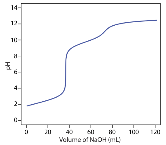
Figure \(\PageIndex{16}\) shows the potentiometric titration curve for the titration of a 0.500-g sample an unknown weak acid. The titrant is 0.1032 M NaOH. What is the weak acid’s equivalent weight?
- Answer
-
The first of the two visible end points is approximately 37 mL of NaOH. The analyte’s equivalent weight, therefore, is
\[(0.1032 \ \mathrm{M} \ \mathrm{NaOH})(0.037 \ \mathrm{L}) \times \frac{1 \text { equivalent }}{\mathrm{mol} \ \mathrm{NaOH}}=3.8 \times 10^{-3} \text { equivalents } \nonumber\]
\[E W=\frac{0.5000 \ \mathrm{g}}{3.8 \times 10^{-3} \text { equivalents }}=1.3 \times 10^{2} \ \mathrm{g} / \mathrm{equivalent} \nonumber\]
Equilibrium Constants
Another application of acid–base titrimetry is the determination of a weak acid’s or a weak base’s dissociation constant. Consider, for example, a solution of acetic acid, CH3COOH, for which the dissociation constant is
\[K_{\mathrm{a}}=\frac{\left[\mathrm{H}_{3} \mathrm{O}^{+}\right]\left[\mathrm{CH}_{3} \mathrm{COO}^{-}\right]}{\left[\mathrm{CH}_{3} \mathrm{COOH}\right]} \nonumber\]
When the concentrations of CH3COOH and CH3COO– are equal, the Ka expression reduces to Ka = [H3O+], or pH = pKa. If we titrate a solution of acetic acid with NaOH, the pH equals the pKa when the volume of NaOH is approximately 1⁄2Veq. As shown in Figure \(\PageIndex{17}\), a potentiometric titration curve provides a reasonable estimate of acetic acid’s pKa.
Recall that pH = pKa is a step on a ladder diagram, which divides the pH axis into two regions, one where the weak acid is the predominate species, and one where its conjugate weak base is the predominate species.
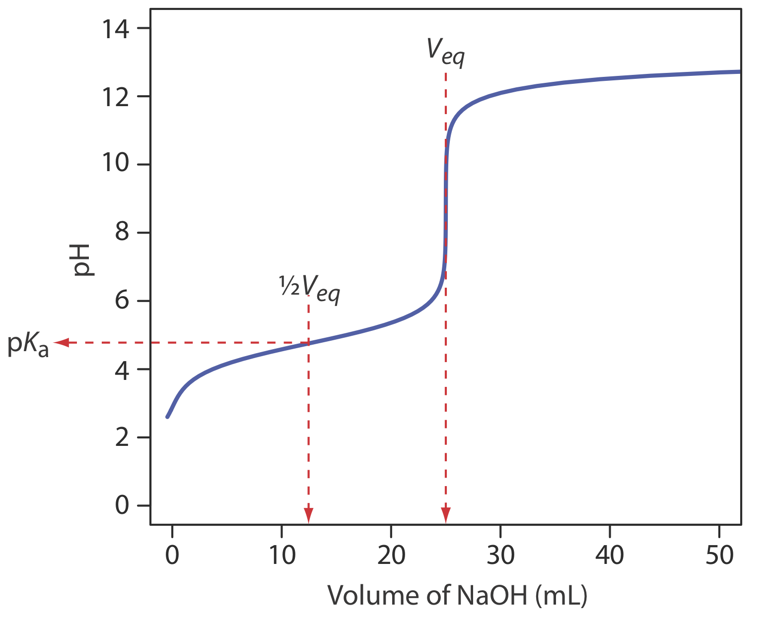
This method provides a reasonable estimate for a weak acid’s pKa if the acid is neither too strong nor too weak. These limitations are easy to appreciate if we consider two limiting cases. For the first limiting case, let’s assume the weak acid, HA, is more than 50% dissociated before the titration begins (a relatively large Ka value); in this case the concentration of HA before the equivalence point is always less than the concentration of A– and there is no point on the titration curve where [HA] = [A–]. At the other extreme, if the acid is too weak, then less than 50% of the weak acid reacts with the titrant at the equivalence point. In this case the concentration of HA before the equivalence point is always greater than that of A–. Determining the pKa by the half-equivalence point method overestimates its value if the acid is too strong and underestimates its value if the acid is too weak.
Use the potentiometric titration curve in Figure \(\PageIndex{16}\) to estimate the pKa values for the weak acid in Exercise \(\PageIndex{10}\).
- Answer
-
At 1⁄2Veq, or approximately 18.5 mL, the pH is approximately 2.2; thus, we estimate that the analyte’s pKa is 2.2.
A second approach for determining a weak acid’s pKa is to use a Gran plot. For example, earlier in this chapter we derived the following equation for the titration of a weak acid with a strong base.
\[\left[\mathrm{H}_{3} \mathrm{O}^{+}\right] \times V_{b}=K_{a} V_{e q}-K_{a} V_{b} \nonumber\]
A plot of [H3O+] \(\times\) Vb versus Vb for volumes less than the equivalence point yields a straight line with a slope of –Ka. Other linearizations have been developed that use the entire titration curve or that require no assumptions [(a) Gonzalez, A. G.; Asuero, A. G. Anal. Chim. Acta 1992, 256, 29–33; (b) Papanastasiou, G.; Ziogas, I.; Kokkindis, G. Anal. Chim. Acta 1993, 277, 119–135]. This approach to determining an acidity constant has been used to study the acid–base properties of humic acids, which are naturally occurring, large molecular weight organic acids with multiple acidic sites. In one study a humic acid was found to have six titratable sites, three which were identified as carboxylic acids, two which were believed to be secondary or tertiary amines, and one which was identified as a phenolic group [Alexio, L. M.; Godinho, O. E. S.; da Costa, W. F. Anal. Chim. Acta 1992, 257, 35–39].
Values of Ka determined by this method may have a substantial error if the effect of activity is ignored. See Chapter 6.9 for a discussion of activity.
Evaluation of Acid–Base Titrimetry
Scale of Operation
In an acid–base titration, the volume of titrant needed to reach the equivalence point is proportional to the moles of titrand. Because the pH of the titrand or the titrant is a function of its concentration, the change in pH at the equivalence point—and thus the feasibility of an acid–base titration—depends on their respective concentrations. Figure \(\PageIndex{18}\), for example, shows a series of titration curves for the titration of several concentrations of HCl with equimolar solutions NaOH. For titrand and titrant concentrations smaller than 10–3 M, the change in pH at the end point is too small to provide an accurate and a precise result.
Acid–base titrimetry is an example of a total analysis technique in which the signal is proportional to the absolute amount of analyte. See Chapter 3 for a discussion of the difference between total analysis techniques and concentration techniques.
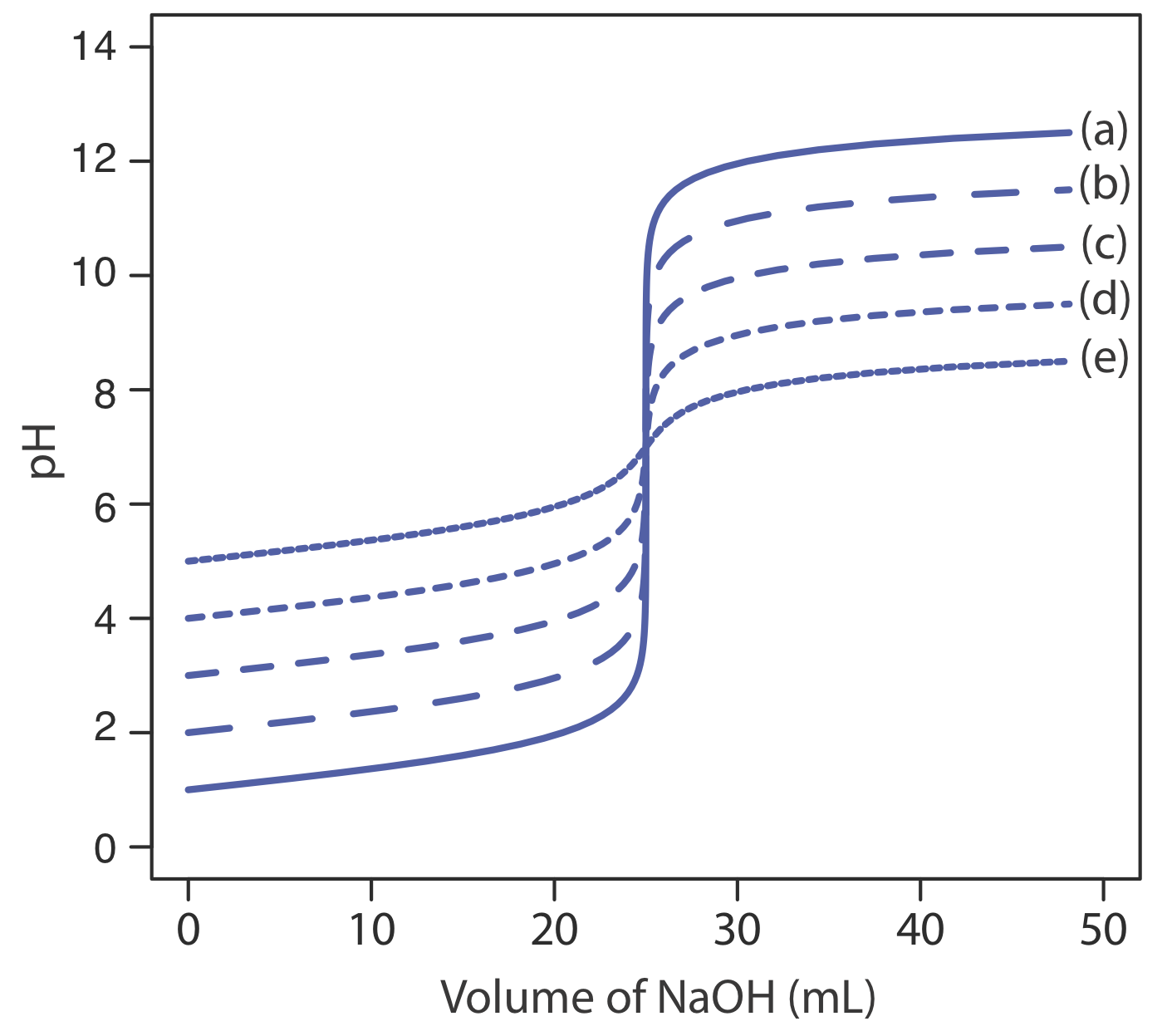
A minimum concentration of 10–3 M places limits on the smallest amount of analyte we can analyze successfully. For example, suppose our analyte has a formula weight of 120 g/mol. To successfully monitor the titration’s end point using an indicator or a pH probe, the titrand needs an initial volume of approximately 25 mL. If we assume the analyte’s formula weight is 120 g/mol, then each sample must contain at least 3 mg of analyte. For this reason, acid–base titrations generally are limited to major and minor analytes. We can extend the analysis of gases to trace analytes by pulling a large volume of the gas through a suitable collection solution.
We need a volume of titrand sufficient to cover the tip of the pH probe or to allow for an easy observation of the indicator’s color. A volume of 25 mL is not an unreasonable estimate of the minimum volume.
One goal of analytical chemistry is to extend analyses to smaller samples. Here we describe two interesting approaches to titrating μL and pL samples. In one experimental design (Figure \(\PageIndex{19}\)), samples of 20–100 μL are held by capillary action between a flat-surface pH electrode and a stainless steel sample stage [Steele, A.; Hieftje, G. M. Anal. Chem. 1984, 56, 2884–2888]. The titrant is added using the oscillations of a piezoelectric ceramic device to move an angled glass rod in and out of a tube connected to a reservoir that contains the titrant. Each time the glass tube is withdrawn an approximately 2 nL microdroplet of titrant is released. The microdroplets are allowed to fall onto the sample, with mixing accomplished by spinning the sample stage at 120 rpm. A total of 450 microdroplets, with a combined volume of 0.81–0.84 μL, is dispensed between each pH measurement. In this fashion a titration curve is constructed. This method has been used to titrate solutions of 0.1 M HCl and 0.1 M CH3COOH with 0.1 M NaOH. Absolute errors ranged from a minimum of +0.1% to a maximum of –4.1%, with relative standard deviations from 0.15% to 4.7%. Samples as small as 20 μL were titrated successfully.
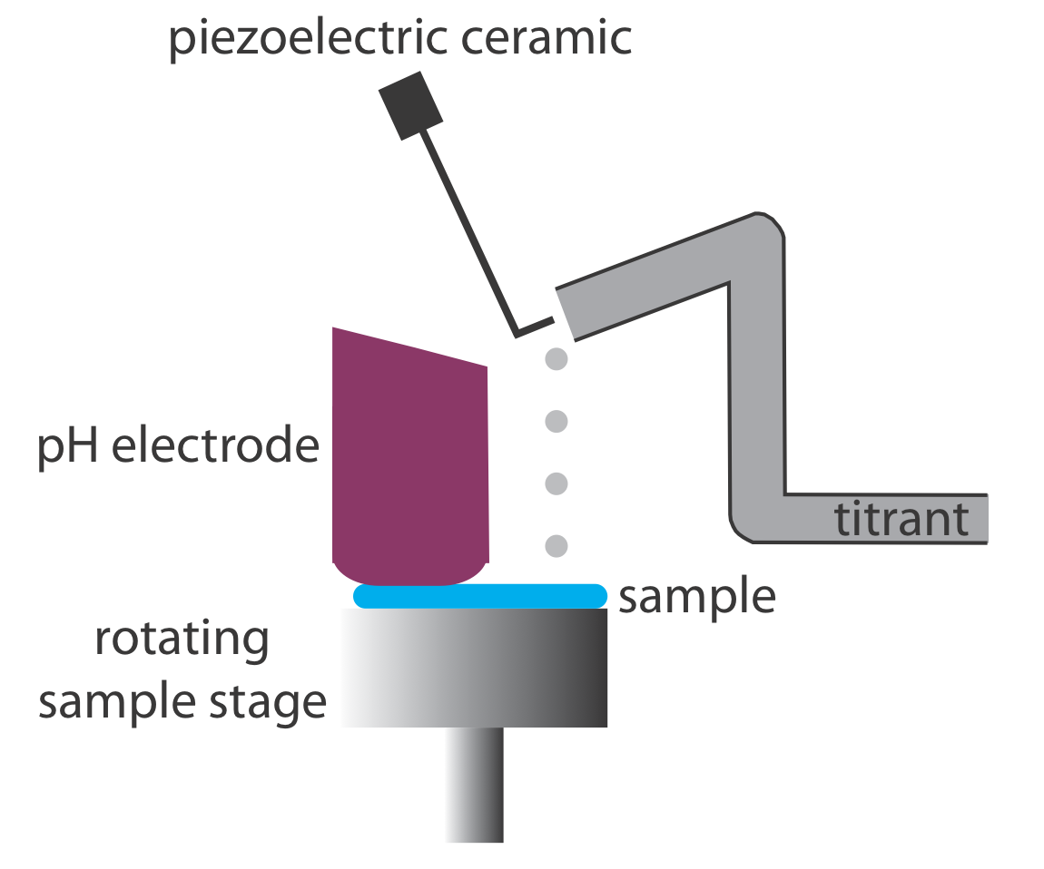
Another approach carries out the acid–base titration in a single drop of solution [(a) Gratzl, M.; Yi, C. Anal. Chem. 1993, 65, 2085–2088; (b) Yi, C.; Gratzl, M. Anal. Chem. 1994, 66, 1976–1982; (c) Hui, K. Y.; Gratzl, M. Anal. Chem. 1997, 69, 695–698; (d) Yi, C.; Huang, D.; Gratzl, M. Anal. Chem. 1996, 68, 1580–1584; (e) Xie, H.; Gratzl, M. Anal. Chem. 1996, 68, 3665–3669]. The titrant is delivered using a microburet fashioned from a glass capillary micropipet (Figure \(\PageIndex{20}\)). The microburet has a 1-2 μm tip filled with an agar gel membrane. The tip of the microburet is placed within a drop of the sample solution, which is suspended in heptane, and the titrant is allowed to diffuse into the sample. The titration’s progress is monitored using an acid–base indicator and the time needed to reach the end point is measured. The rate of the titrant’s diffusion from the microburet is determined by a prior calibration. Once calibrated the end point time is converted to an end point volume. Samples usually consist of picoliter volumes (10–12 liters), with the smallest sample being 0.7 pL. The precision of the titrations is about 2%.
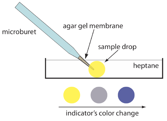
Titrations conducted with microliter or picoliter sample volumes require a smaller absolute amount of analyte. For example, diffusional titrations have been conducted on as little as 29 femtomoles (10–15 moles) of nitric acid. Nevertheless, the analyte must be present in the sample at a major or minor level for the titration to give accurate and precise results.
Accuracy
When working with a macro–major or a macro–minor sample, an acid–base titration can achieve a relative error of 0.1–0.2%. The principal limitation to accuracy is the difference between the end point and the equivalence point.
Precision
An acid–base titration’s relative precision depends primarily on the precision with which we can measure the end point volume and the precision in detecting the end point. Under optimum conditions, an acid–base titration has a relative precision of 0.1–0.2%. We can improve the relative precision by using the largest possible buret and by ensuring we use most of its capacity in reaching the end point. A smaller volume buret is a better choice when using costly reagents, when waste disposal is a concern, or when we must complete the titration quickly to avoid competing chemical reactions. An automatic titrator is particularly useful for titrations that require small volumes of titrant because it provides significantly better precision (typically about ±0.05% of the buret’s volume).
The precision of detecting the end point depends on how it is measured and the slope of the titration curve at the end point. With an indicator the precision of the end point signal usually is ±0.03–0.10 mL. Potentiometric end points usually are more precise.
Sensitivity
For an acid–base titration we can write the following general analytical equation to express the titrant’s volume in terms of the amount of titrand
\[\text { volume of titrant }=k \times \text { moles of titrand } \nonumber\]
where k, the sensitivity, is determined by the stoichiometry between the titrand and the titrant. Consider, for example, the determination of sulfurous acid, H2SO3, by titrating with NaOH to the first equivalence point
\[\mathrm{H}_{2} \mathrm{SO}_{3}(a q)+\mathrm{OH}^{-}(a q) \rightarrow \mathrm{H}_{2} \mathrm{O}(l )+\mathrm{HSO}_{3}^{-}(a q) \nonumber\]
At the equivalence point the relationship between the moles of NaOH and the moles of H2SO3 is
\[\mathrm{mol} \ \mathrm{NaOH}=\mathrm{mol} \ \mathrm{H}_{2} \mathrm{SO}_{3} \nonumber\]
Substituting the titrant’s molarity and volume for the moles of NaOH and rearranging
\[M_{\mathrm{NaOH}} \times V_{\mathrm{NNOH}}=\mathrm{mol} \ \mathrm{H}_{2} \mathrm{SO}_{3} \nonumber\]
\[V_{\mathrm{NaOH}}=\frac{1}{M_{\mathrm{NaOH}}} \times \mathrm{mol} \ \mathrm{H}_{2} \mathrm{SO}_{3} \nonumber\]
we find that k is
\[k=\frac{1}{M_{\mathrm{NaOH}}} \nonumber\]
There are two ways in which we can improve a titration’s sensitivity. The first, and most obvious, is to decrease the titrant’s concentration because it is inversely proportional to the sensitivity, k. The second approach, which applies only if the titrand is multiprotic, is to titrate to a later equivalence point. If we titrate H2SO3 to its second equivalence point
\[ \mathrm{H}_{2} \mathrm{SO}_{3}(a q)+2 \mathrm{OH}^{-}(a q) \rightarrow 2 \mathrm{H}_{2} \mathrm{O}(l)+\mathrm{SO}_{3}^{2-}(a q)\nonumber\]
then each mole of H2SO3 consumes two moles of NaOH
\[\mathrm{mol} \ \mathrm{NaOH}=2 \times \mathrm{mol} \ \mathrm{H}_{2} \mathrm{SO}_{3} \nonumber\]
and the sensitivity becomes
\[k=\frac{2}{M_{\mathrm{NaOH}}} \nonumber\]
In practice, however, any improvement in sensitivity is offset by a decrease in the end point’s precision if a larger volume of titrant requires us to refill the buret. For this reason, standard acid–base titrimetric procedures are written to ensure that a titration uses 60–100% of the buret’s volume.
Selectivity
Acid–base titrants are not selective. A strong base titrant, for example, reacts with all acids in a sample, regardless of their individual strengths. If the titrand contains an analyte and an interferent, then selectivity depends on their relative acid strengths. Let’s consider two limiting situations.
If the analyte is a stronger acid than the interferent, then the titrant will react with the analyte before it begins reacting with the interferent. The feasibility of the analysis depends on whether the titrant’s reaction with the interferent affects the accurate location of the analyte’s equivalence point. If the acid dissociation constants are substantially different, the end point for the analyte can be determined accurately. Conversely, if the acid dissociation constants for the analyte and interferent are similar, then there may not be an accurate end point for the analyte. In the latter case a quantitative analysis for the analyte is not possible.
In the second limiting situation the analyte is a weaker acid than the interferent. In this case the volume of titrant needed to reach the analyte’s equivalence point is determined by the concentration of both the analyte and the interferent. To account for the interferent’s contribution to the end point, an end point for the interferent must be available. Again, if the acid dissociation constants for the analyte and interferent are significantly different, then the analyte’s determination is possible. If the acid dissociation constants are similar, however, there is only a single equivalence point and we cannot separate the analyte’s and the interferent’s contributions to the equivalence point volume.
Time, Cost, and Equipment
Acid–base titrations require less time than most gravimetric procedures, but more time than many instrumental methods of analysis, particularly when analyzing many samples. With an automatic titrator, however, concerns about analysis time are less significant. When performing a titration manually our equipment needs—a buret and, perhaps, a pH meter—are few in number, inexpensive, routinely available, and easy to maintain. Automatic titrators are available for between $3000 and $10 000.