1.3: Converting Units-Dimensional Analysis

Learning Objectives

• Convert a value reported in one unit to a corresponding value in a different unit.

The ability to convert from one unit to another is an important skill. For example, a nurse with 50 mg aspirin tablets who must administer 0.2 g of aspirin to a patient needs to know that 0.2 g equals 200 mg, so 4 tablets are needed. Fortunately, there is a simple way called dimensional analysis to convert from one unit to another. Dimensional analysis uses convesion factors.

Conversion Factors

Here is a simple example. How many centimeters are there in 3.55 m?

The relationship between cm and m is shown below:

\[100\; \rm{cm} = 1\; \rm{m} \nonumber \]

From this relationship we can derive two conversion factors:

A fraction that has equivalent quantities in the numerator and the denominator but expressed in different units is called a conversion factor.

To solve the problem we use one of the two conversion factors. We first write the quantity we are given, 3.55 m. Then we multiply this quantity by conversion factor # 1.

\[ 3.55 \; \rm{m} \times \dfrac{100 \; \rm{cm}}{1\; \rm{m}} \nonumber \]

Conversion factor # 1 is chosen because m, the abbreviation for meters, occurs in both the numerator and the denominator of our expression, they cancel out. The final step is to perform the calculation that remains once the units have been canceled. We find that 3.55 m equals 355 cm.

A generalized description of this process is as follows:

\[\text{quantity (in old units)} \times \text{conversion factor} = \text{quantity (in new units)} \nonumber \]

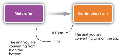
If you can master the technique of applying conversion factors, you will be able to solve a large variety of problems. Figure \(\PageIndex{1}\) shows a concept map for constructing a proper conversion.

Figure \(\PageIndex{1}\): A Concept Map for Conversions. This is how you construct a conversion factor to convert from one unit to another.

Meters is converted to centimeters. In the fraction showing 100 cm over 1 m, the unit you convert to is on top, and the unit you convert from is on bottom.

Significant Figures in Conversions

How do conversion factors affect the determination of significant figures? Numbers in conversion factors based on prefix changes, such as meters to centimeters, are not considered in the determination of significant figures in a calculation because the numbers in conversion factors are exact. Exact numbers are defined or counted numbers, (not measured numbers), and can be considered as having an infinite number of significant figures. (In other words, 1 m is exactly 100 cm, by the definition of centi-.) Counted numbers are also exact. If there are 16 students in a classroom, the number 16 is exact. In contrast, conversion factors that come from measurements (such as density, as we will see shortly) are approximations have a limited number of significant figures and should be considered in determining the significant figures of the final answer.

Example \(\PageIndex{1}\)

1. The average volume of blood in an adult male is 4.7 L. What is this volume in milliliters?
2. A hummingbird can flap its wings once in 18 ms. How many seconds are in 18 ms?

Solution

1. We start with what we are given, 4.7 L. We want to change the unit from liters to milliliters. There are 1,000 mL in 1 L. From this relationship, we can construct two conversion factors:

\[ \dfrac{1\; \rm{L}}{1,000\; \rm{mL}} \; \text{ or } \; \dfrac{1,000 \; \rm{mL}}{1\; \rm{L}} \nonumber \]

We use the conversion factor that will cancel out the original unit, liters, and introduce the unit we are converting to, which is milliliters. The conversion factor that does this is the one on the right.

\[ 4.7 \cancel{\rm{L}} \times \dfrac{1,000 \; \rm{mL}}{1\; \cancel{\rm{L}}} = 4,700\; \rm{mL} \nonumber \]

Because the numbers in the conversion factor are exact, we do not consider them when determining the number of significant figures in the final answer. Thus, we report two significant figures in the final answer.

2. We can construct two conversion factors from the relationships between milliseconds and seconds:

\[ \dfrac{1,000 \; \rm{ms}}{1\; \rm{s}} \; \text{ or } \; \dfrac{1\; \rm{s}}{1,000 \; \rm{ms}} \nonumber \]

To convert 18 ms to seconds, we choose the conversion factor that will cancel out milliseconds and introduce seconds. The conversion factor on the right is the appropriate one. We set up the conversion as follows:

\[ 18 \; \cancel{\rm{ms}} \times \dfrac{1\; \rm{s}}{1,000 \; \cancel{\rm{ms}}} = 0.018\; \rm{s} \nonumber \]

The conversion factor’s numerical values do not affect our determination of the number of significant figures in the final answer.

Exercise \(\PageIndex{1}\)

Perform each conversion.

1. 101,000 ns to seconds
2. 32.08 kg to grams

Answer a

\[ 101,000 \cancel{\rm{ns}} \times \dfrac{1\; \rm{s}}{1,000,000,000\; \cancel{\rm{ns}}} = 0.000101\; \rm{s} \nonumber \]

Answer b

\[ 32.08 \cancel{\rm{kg}} \times \dfrac{1,000 \; \rm{g}}{1\; \cancel{\rm{kg}}} = 32,080\; \rm{g} \nonumber \]

Concept Review Exercises

1. How do you determine which quantity in a conversion factor goes in the denominator of the fraction?
2. State the guidelines for determining significant figures when using a conversion factor.

Answers

1. The unit you want to cancel from the numerator goes in the denominator of the conversion factor.
2. Exact numbers that appear in many conversion factors do not affect the number of significant figures; otherwise, the normal rules of multiplication and division for significant figures apply.

Key Takeaway

• A unit can be converted to another unit of the same type with a conversion factor.