
Properties of the solutions to the Schrödinger equation
- Page ID
- 1696
Beginning in the early 20th century, physicists began to acknowledge that matter--much like electromagnetic radiation--possessed wave-like behaviors. While electromagnetic radiation were well understood to obey Maxwell's Equations, matter obeyed no known equations.
Introduction
In 1926, the Austrian physicist Erwin Schrödinger formulated what came to be known as the Schrödinger Equation:
\[ i\hbar\dfrac{\partial}{\partial t}\psi(x,t)=\dfrac{-\hbar}{2m}\nabla^2\psi(x,t) +V(x)\psi(x,t) \label{1.1}\]
Equation \ref{1.1} effectively describes matter as a wave that fluctuates with both displacement and time. However, in most applications of the wave behavior of matter, we are only interested in the probability of finding the particle in a particular region. This probability in a one dimensional system is defined as:
\[\int\psi(x,t)^*\psi(x,t)dxdt\label{1.2}\]
Equation \ref{1.2} describes the probability of finding a particle as the integral of the wavefunction times its complex conjugate. The complex conjugate is effective in that it negates all imaginary components of the wavefunction. Since the imaginary portion of the equation dictates its time dependence, it is sufficed to say that for most purposes it can be treated as time-independent. The result is seen in Equation \ref{1.3}:
\[\dfrac{-\hbar^2}{2m}\dfrac{d^2\psi(x)}{dx^2}+V(x)\psi(x) = E\psi(x) \label{1.3}\]
Although this time-independent Schrödinger equation can be useful to describe a matter wave in free space, we are most interested in waves when confined to a small region, such as an electron confined in a small region around the nucleus of an atom. Several different models have been developed that provide a means by which to study a matter-wave when confined to a small region: the particle in a box (infinite well), finite well, and the Hydrogen atom. We will discuss each of these in order to develop a greater understanding for how a wave behaves when it is in a bound state.
The Particle in a One Dimensional Box (The Infinite Well)
The particle in a box is a very simple model developed in order to understand the behavior of a particle (i.e. an electron) when confined to a small region of length, L, with infinite potential barriers, V, at x=0 and x=L, as seen in Figure 1.
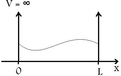
When a particle of wavelength λ is placed in a box with length L ≈ λ, the particle begins to exhibit significant wave-like characteristics, as seen in Figure 1.
Now, in this model, we first assume that the particle has zero potential energy and is bound in a well with barriers of infinite potential energy. Therefore, we may negate the potential energy, V, component of Equation \ref{1.3}:
\[\dfrac{-\hbar^2}{2m}\frac{d^2\psi(x)}{dx^2} = E\psi(x) \label{1.4}\]
Now, if we rearrange Equation \ref{1.4}, we obtain:
\[\frac{d^2\psi(x)}{dx^2} = \dfrac{-2mE}{\hbar^2}\psi(x) \label{1.5}\]
Equation \ref{1.5} is a second order differential equation, in which we are interested in solving for Ψ and E. Looking at Equation \ref{1.4}, we see that we have a wavefunction, Ψ, whose second derivative is equal to the negative of itself times some constants. This means that Ψ must be a trigonometric function, represented as:
\[\psi(x) = A\sin(kx) + B\cos(kx) \label{1.6}\]
Next, we mandate that the wavefunction be continuous. Since we have infinite potential energy barriers, there is zero probability that the particle would be found at x<0 or x>L. Therefore, we must have Ψ(0)=0 and Ψ(L)=0. Applying these conditions to Equation \ref{1.6}, we have
\[0 = \psi(0) = A\sin(0) + B\cos(0)\]
Because cos(0)≠ 0, we must have B=0, so this means that Ψ cannot involve a cosine function. Thus, Equation \ref{1.6} may be reduced to
\[\psi(x) = Asin(kx) \label{1.7}\]
We now differentiate \(\psi(x)\) twice to solve for k; we obtain
\[\frac{d\psi(x)}{dx} = kAcos(kx)\]
\[\frac{d^2\psi(x)}{dx^2} = -k^2Asin(kx)\]
\[\frac{d^2\psi(x)}{dx^2} = -k^2\psi(x) \label{1.8}\]
Now if we relate Equation \ref{1.5} to Equation \ref{1.8}, we have
\[k^2 = \frac{2mE}{\hbar^2}\]
\[k = \frac{\sqrt{2mE}}{\hbar} \label{1.9}\]
Because the wavefunction is limited in the confines of the infinite well, the wavenumber, k, can only take on certain discrete values that would allow Ψ(0)=0 and Ψ(L)=0. Therefore, it is found that
\[k=\frac{n\pi}{L} \label{1.10}\]
where L is the length of the well and n is the energy level or fundamental quantum number of the particle in the well. If we now set Equation 1.9 equal to Equation 1.10 and solve for the energy we obtain
\[E=\frac{n^2\pi^2\hbar^2}{2mL^2} \label{1.11}\]
Equation \ref{1.11} is a very useful equation because it relates the energy of a particle in a system to the size of its confines, L, its mass, m, and its energy level, n.
Now that we have solved for the Energy of a particle in an infinite well, we can return to solving for the wavefunction Ψ(x). By substituting Equation 1.10 into Equation 1.7, we will have
\[\psi(x) = Asin(\frac{n\pi x}{L}) \label{1.12}\]
Finally in order to solve for A, we can apply the condition of normalizability; that is, the probability of finding the wavefunction between x=0 and x=L must be equal to unity. So, we have
\[1=\int \psi^2(x)dx=\int (Asin(\frac{n\pi x}{L}))^2dx \label{1.13}]
Equation \ref{1.13} can be used to solve for the normalization constant, A, while making use of the identity wherein \(sin^2(ax)= \frac{x}{2} - \frac{sin(2ax)}{4a}\). We will get
\[|A|=\sqrt{\frac{2}{L}}\]
Therefore, we can now rewrite Equation \ref{1.10} as
\[\psi(x) = \sqrt{\frac{2}{L}}sin(\frac{n\pi x}{L}) \label{1.14}\]
We now have solved the Schrödinger Equation for the Particle in a Box, and can apply Equations \ref{1.11} and \ref{1.14}, which describe the wavefunction, Ψ, and the energy, E, respectively, to many applications, especially when trying to understand the behaviors of quantum mechanical particles in small confines (i.e. an electron orbiting a nucleus).
Particle in a Finite Well
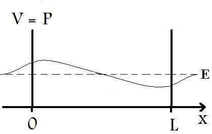
What distinguishes the Finite Well from the Particle in a Box scenarios are that for the finite well, the potential energy, V, of the barriers do not approach infinity. As a result, we find that the particle is not totally restricted to the region between the barrier, as shown in Figure 2 below.
In solving the Schrödinger Equation for the Finite Well, we cannot apply some of the same conditions that were imposed on the Particle in a Box; in fact, the Schrödinger Equation for a Finite Well cannot be solved exactly, but must employ numeric approximations. However, it is still useful to show the basic functions that describe the wave-like particle. So, we must reapply the same methodology that we used for the Particle in a Box. For the region between x=0 and x=L, we have a potential energy, V, equal to zero. Thus, the time-independent Schrödinger Equation can be reduced to
\(\frac{-\hbar^2}{2m}\frac{d^2\psi(x)}{dx^2} = E\psi(x)\) (2.1)
Moreover for this region inside the box, we again find that the wavefunction is defined as
\(\psi(x) = Asin(kx) + Bcos(kx)\) (2.2)
However, we can no longer utilize the same barrier conditions to remove the cosine portion of the wavefunction. So, we will not be able to solve it further without numerical approximations. We can, however, make use of our result in the derivations for the Particle in a Box to obtain a formula for the Energy of a particle in a Finite Well. From Equation , we have
\(k = \frac{\sqrt{2mE}}{\hbar}\) (2.3)
Therefore, we obtain
\(E=\frac{k^2\hbar^2}{2m}\) (2.4)
For the regions outside the well, x<0 and x>L, we cannot employ the same analysis we used earlier because the potential energy,V, is not infinite but equal to a constant, P. Therefore, we will again solve the regions outside the potential well beginning with the time-independent Schrödinger Equation
\(\dfrac{-\hbar^2}{2m}\frac{d^2\psi(x)}{dx^2}+V(x)\psi(x) = E\psi(x)\) (2.5)
For these regions outside the well, we have the potential energy V(x) = P. Therefore, Equation 2.5 may be rewritten as
\(\dfrac{-\hbar^2}{2m}\frac{d^2\psi(x)}{dx^2}+P\psi(x) = E\psi(x)\) (2.6)
Rearranging we have
\(\dfrac{d^2\psi(x)}{dx^2} = \frac{2m(P-E)\psi(x)}{\hbar^2}\) (2.7)
Now, for the regions outside the well, the particle may have energy that is greater than or less than the potential energy of the well. Where, E>P, the particle is said to be in a free state and we again find that
\(k = \dfrac{\sqrt{2m(E-P)}}{\hbar}\) (2.8)
and where E<P, the particle is said to be in a bound state and we define
\(\alpha = \dfrac{\sqrt{2m(P-E)}}{\hbar}\) (2.9)
In order to describe the wavefunction in the regions outside the well, a closer examination of Equation 2.7 is needed. We have a second order differential equation where the second derivative of the wavefunction, Ψ(x), is equal the positive of the wavefunction times some constants. Trigonometric functions do not satisfy this condition, but exponentials do. Thus, we have
\(\psi(x) = Ce^{-\alpha x} + De^{\alpha x}\) (2.10)
Now, referring back to Figure 2, we see that in the region, where 0<x<L, the function takes on a trigonometric form. In the region where x<0, we see that as x goes to -∞, the C term goes to infinity. Since, the wavefunction must have a finite total integral, the C term must be negated; so we have
\(\psi(x) = De^{\alpha x}\) where x<0. (2.11)
By the same condition, we see that for the region where x>L, as x goes to ∞, the D term goes to infinity. As a result, this D term must be negated. Thus, we have
\(\psi(x) = Ce^{-\alpha x}\) where x>L (2.12)
Solving for the constants, C and D, is not possible without numerical approximations, so we will be sufficed with Equations 2.11 and 2.12 as descriptions of the wavefunction, Ψ, in the regions outside the Finite Well.
The Hydrogen Atom
The solutions to the Infinite Well and Finite Well are useful for describing the behavior of a particle when confined to a small region of space with large and small potential barriers, respectively. However, this one dimensional treatment of the displacement of a particle in space does not provide a comprehensive understanding of the behavior of an electron orbiting a nucleus (i.e. a hydrogen atom). Beginning with Equation 1.1, we can describe the wavefunction in terms of the three dimensions, x, y, and z, as follows
\]\frac{-\hbar^2}{2m_e}[\frac{\partial^2\psi}{\partial x^2} + \frac{\partial^2\psi}{\partial y^2} +\frac{\partial^2\psi}{\partial z^2}] + V(x,y,z)\psi(x,y,z) = E\psi(x,y,z) \label{3.1\]
Treatment of Equation 3.1 in Spherical Polar Coordinates significantly facilitates the problem. So, after some rearranging, we have
\[\frac{\partial^2\psi}{\partial r^2} + \frac{2}{r}\frac{\partial\psi}{\partial r} + \frac{1}{r^2sin\theta}\frac{\partial[sin\theta(\partial\psi/\partial\theta)]}{\partial\theta} + \frac{1}{r^2 sin\theta}\frac{\partial^2\psi}{\partial\phi^2} + \frac{2m_e}{\hbar^2}(E+\frac{e^2}{4\pi\epsilon_0 r})\psi = 0 \label{3.2}\]
Equation 3.2 provides a very complex description for the wavefunction of an electron orbiting in a Hydrogen Atom. Fortunately, it has already been solved, and so we will simply examine the solutions. But first, it is important to note that the wavefunction can be described as the product of three distinct functions
\[\psi(r,\theta,\phi) = R(r)\Theta(\theta)\Phi(\phi)\label{3.3}]
where \(R(r)\) is the radial part and \(\Theta(\theta)\Phi(\phi)\) is the angular part. A deeper analysis of Equation \ref{3.2} reveals three quantum numbers, \(n\), \(l\), and \(m_l\). The fundamental quantum number,\(n\), describes the size of the orbital in which the electron orbits. The angular momentum quantum number, \(l\), describes the shape of the orbital. Finally, the magnetic quantum number, \(m_l\), describes the orientation of the orbital in space.
Now, for any given value of n (n = 1,2,3,...), there are n values of l, which are given by l = 0,1,2,...,(n-1). While, the magnetic quantum number, \(m_l\), takes on values of \(m_l\)=0, \(\pm\)1, \(\pm\)2,...\(\pm l\).
A more in-depth analysis of Equation 3.2, which is beyond the scope of this module, allows for a derivation of the energy of an electron in a Hydrogen atom. We will just make use of the result where
\[E_n = -hcR_H (\frac{1}{n^2}); n =1,2,3,... \label{3.4}\]
or
\[E_n = -13.6eV (\frac{1}{n^2}) ; n =1,2,3,...\label{3.5}\]
As Equations \ref{3.4} and \ref{3.5} show, the energy of an electron in a Hydrogen atom is only dependent on the fundamental quantum number, n. This is not the case for more complex atoms, whose energy also depends on the angular momentum quantum number, \(l\).
By solving the Schrödinger Equation for the Infinite Well, Finite Well, and the Hydrogen Atom, we are able to establish models that allow for a good understanding of the behavior of a particle when confined to a small region of space, whose length is proportional to the Planck wavelength of the particle. By restricting the particle to portential wells, we are able to derive the particle's wavefunction--both inside and outside of the well--and the quantum mechanical energy that the particle possesses due to its wave-like behavior.
Problems
1. Calculate the ground state energy of a baseball that weighs 145 grams that is in a football field 100 yards long.
Solution:
We have m = 0.145 kg and L = \(100yards(\frac{0.9144meter}{1 yard} = 91.44meters\)
Plugging these values into Equation 1.11, we have
\[E_{baseball}=\dfrac{1^2\pi^2(1.05x10^{-34})^2}{2(0.145)(91.44)^2}= 4.49x10^{-71}J\]
2. Calculate the energy of an electron in a well that is 1 Å long.
Solution:
We apply the same technique as in Problem 1
\[E_{electron}=\dfrac{1^2\pi^2(1.05x10^{-34})^2}{2(9.11x10^{-31})(1x10^{-10})^2}= 5.69x10^{16}J\]
Note: It is important to realize that in the case of the baseball in a football field, the quantum mechanical energies associated with its wavelike behavior are so small that they are essetially negligible. This is why we see a continuum of energy associated with its motion, whereas the electron has defined quanta of energy in which it can orbit.
3. Derive the wavefunction, Ψ, and energy, E, for the Particle in a 1 dimensional box (infinite well), while describing any conditions that must be imposed on the wavefunction.
Solution:
Refer to Section 1 above.
4. Find the probability that an electron in the n=2 state of an infinite well (1 Å long) is found between x=L/4 and x=3L/4.
Solution:
Although this problem could be solved by integration as follows
\[P = \int^{3L/4}_{L/4}\psi(x)^2dx\]
where
\[\psi(x) = \sqrt\frac{2}{L}sin(\frac{n\pi}{L}x) \label{P.1} \]
it can be more readily solved by taking a look at the graph of the probability of the wavefunction in an infinite well as seen in Figure P.4 below
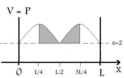
As Figure P.4 shows, we can infer the probability of finding the particular between x=L/4 and x=3L/4 to be P=1/2, simply because of symmetry. This assessment only works for symmetrical wavefunction distributions. For all others, Equation P.1 must be used.
5. For an electron in the n=4 energy level, what values of \(l\) and \(m_l\) are allowed?
Solution:
\(l = 0,1,2, and 3\)
\(m_l = -3,-2,-1,0,1,2,3\)
References
- Chang, Raymond. Physical Chemistry for the Biosciences. Sansalito, CA: University Science, 2005. Print.
- "Finite Potential Well." Wikipedia, the Free Encyclopedia. Web. 13 Mar. 2011. <http://en.Wikipedia.org/wiki/Finite_potential_well>.
Contributors and Attributions
- John Paul Aboubechara, UC Davis 2012