iii) Chemical reactions coupled to electron transfer

Until now, we have mostly considered electron transfer reactions resulting in electrode products that are stable on the time scale of the experiment. In this section, electron transfer reactions that are subject to follow-up homogeneous chemical reactions will be described. The simplest example of such a reaction can be expressed as

\[\mathrm{Ox + \mathit{n}\, e^- \Leftrightarrow Red \xrightarrow{k_c} Z}\]

where Z represents a product which, unlike Red, can no longer be converted back to Ox by direct electron transfer. The value of k_c, the rate constant for the chemical step, determines how quickly Red reacts to form Z. We have encountered this situation before in our discussion of chemical reversibility. Recall that for large values of kc, the redox couple Ox/Red is described as being chemically irreversible on the time scale of the experiment. If k_c is small (or zero), the observed couple will be chemically reversible. For intermediate values of k_c, the couple is said to have limited chemical reversibility.

Cyclic voltammetry is an excellent technique to probe chemical changes that occur as a result of electron transfer. For reactions that are not completely chemically reversible, the current observed on the return scan will be diminished. Further, since scan rate can be controlled in CV, it is possible in many cases to increase ν until the follow-up step is outrun. In this way, the value of k_c can often be determined.

Many combinations of electron transfer and chemical reaction steps are possible. Electrochemists often use a shorthand notation to describe these various electrode processes, denoting an electron transfer step as “E” and chemical steps, either before or after electron transfer, as “C”. Subscripts allow further differentiation, such as E_r for a reversible electron transfer, and E_i for an irreversible one. The most commonly encountered of these electrode mechanisms will be described here.

E_rC_i Mechanism

The mechanism considered above is classified as E_rC_i, with an electrochemically reversible electron transfer, followed by a chemically irreversible homogeneous step to form Z. In this case, no significant equilibrium exists between Red and Z, and Z is electrochemically inactive in the scanned potential range.

\(\mathbf{E_r}\textrm{: }\mathrm{Ox + ne^- \Leftrightarrow Red}\)

\(\mathbf{C_i}\textrm{: }\mathrm{Red \xrightarrow{k_c} Z}\)

Cyclic voltammograms simulated for various scan rates and a value of k_c = 10 s^-1 are shown below. At the slower scan rates, enough time elapses between the initiation of Ox reduction and the reoxidation of Red to allow complete conversion to Z, and no return oxidation is seen. For fast scan rates, the follow-up step can be outrun, and all Red is reconverted to Ox on the return scan. Between the extremes of slow and fast scan rate, values of (i_p,r / i_p,f) increase from zero to unity. Theoretical working curves can be used to calculate the value of the rate constant, k_c, from the observed current ratios.⁸ (DigiElch simulation parameters: v = 1 - 10 V/s; A = 0.10 cm²; C_i = 1.0 mol/cm³; D = 1.0 x 10^-5 cm²/s; α = 0.50; k_s = 100 cm/s; K_eq = 10,000; k_c = 10 s^-1)

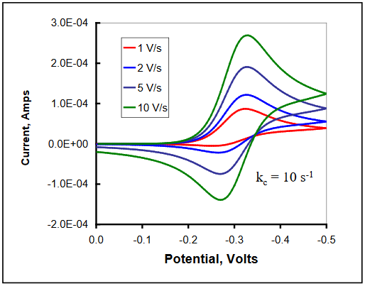
Figure 20

Additional evidence for the presence of this mechanism is an observed shift in the cathodic peak potential (for a reduction) to more positive values as the scan rate is increased. The magnitude of this shift has a theoretical value of (30 / n) mV for each 10x increase in the scan rate.⁹

E_rC_r Mechanism

This mechanism differs from the E_rC_i mechanism in that the chemical step is now reversible, meaning that the concentrations of the reduced form of the redox species, Red, and the product of the chemical step, Z, are maintained at values under equilibrium control.

\(\mathbf{E_r}\textrm{: }\mathrm{Ox + ne^- \Leftrightarrow Red}\)

\(\mathbf{C_r}\textrm{: }\mathrm{Red \Leftrightarrow Z}\)

Thus, the system will be under the control of both the magnitude of the homogeneous rate constant (k_f in this case) and the equilibrium constant K, where K = k_f / k_b. During the return potential scan, the concentration of Red in the vicinity of the electrode becomes smaller as it is converted back to Ox. As this occurs, the equilibrium between Z and Red will try to maintain itself by converting Z into Red. The result is an enhanced anodic peak current at slow to intermediate scan rates (relative to k_f). At very slow scan rates, the peak current ratio, (i_p,r / i_p,f), will approach the chemically reversible value of 1.0. At fast scan rates, the peak current ratio decreases with increasing scan rate, the opposite effect of that observed for the E_rC_i case. Further, for the E_rC_r case, a shift in the cathodic peak potential (for a reduction) to more negative values is observed as the scan rate is increased.

The peak current ratio can be used to distinguish between the two mechanisms. Plots of the current ratio, (i_p,r / i_p,f), as a function of the scan rate for the both the E_rC_i and the E_rC_r cases are shown below. (After Figure 19 in Ref 8.)

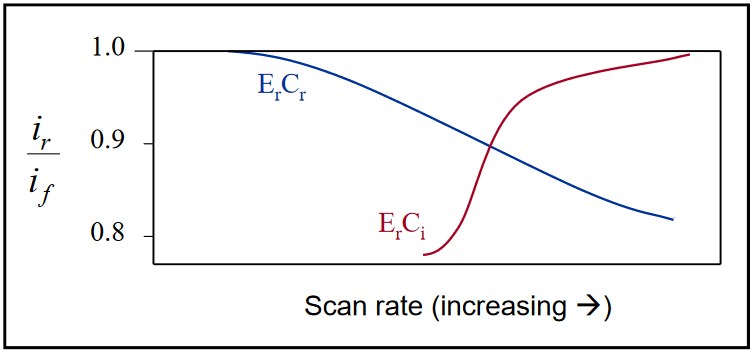
Figure 21

E_rC_i’ Mechanism

In this mechanism, the product of the electrochemical reaction undergoes a chemical reaction with a nonelectroactive solution species to regenerate the starting material. The E_rC_i’ scheme is often referred to as catalytic regeneration.

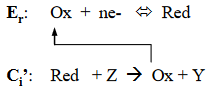
As a first consideration, it will be assumed that Z is present in the solution at a large concentration, representing pseudo first-order conditions. Thus, the regeneration of Ox is controlled by the magnitude of k_c. If k_c is small relative to ν, the observed voltammetry appears reversible, and peak current ratios approach unity. As the magnitude of k_c increases, the amount of Ox that is catalytically regenerated during a potential sweep is increased, with the shape of the corresponding voltammograms transitioning between diffusion control and steady-state behavior. This is illustrated in the Figure22. The same behavior is observed for a single value of k_c as the scan rate is decreased. If scans are continued to potentials well negative of the reduction potential, the limiting currents will converge to the same value regardless of the scan rate as steady-state conditions are reached. (DigiElch simulation parameters: v = 0.10 V/s; A = 0.10 cm²; C_i = 1.0 mol/cm³; D = 1.0 x 10^-5 cm²/s; α = 0.50; k_s = 100 cm/s; large K_eq; k_c = 0.10 - 10 s^-1)

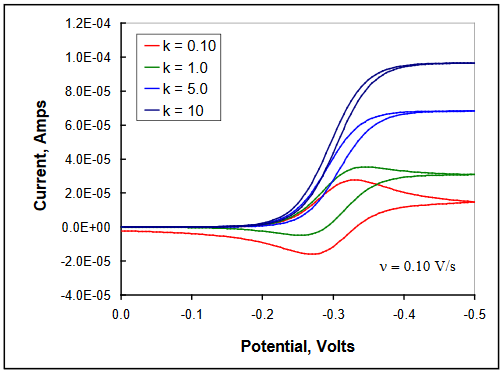
Figure 22

Now consider the case in which the concentration of Z is near to or smaller than that of electrochemically generated Red. Under these conditions, the chemical step becomes true second-order with both concentrations contributing to the kinetics. In the limit as [Z] approaches zero, no chemical step will occur, and reversible voltammetry will be observed. In the region between zero and large [Z], the extent of reaction with Red will increase until the conversion occurs at maximal rate. This effect of increasing [Z] on the observed voltammetry at a single scan rate is illustrated in Figure 23. The value for k_c = 5.0 s^-1 for all scans. (DigiElch simulation parameters: v = 0.10 V/s; A = 0.10 cm²; C_i = 1.0 mol/cm³; D = 1.0 x 10^-5 cm²/s; α = 0.50; k_s = 100 cm/s; large K_eq; k_c = 5.0 s^-1; [Z] = 0.010 – 1.0 M)

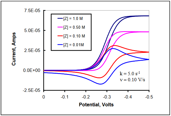
Figure 23

C_rE_r Mechanism

In this mechanism, the electroactive starting material is itself the product of a chemical reaction.

\(\mathbf{C_r}\textrm{: }\mathrm{Z \Leftrightarrow O}\)

\(\mathbf{E_r}\textrm{: }\mathrm{Ox + ne^- \Leftrightarrow Red}\)

The quantity of Ox initially available for reduction is dependent upon the magnitude of the equilibrium constant K between Z and Ox. For large values of K, the equilibrium lies far to the right, favoring the electrochemical species Ox. The observed voltammetry for this case is generally indistinguishable from the chemically reversible case, with peak current ratios approaching unity for all scan rates.

Small values for K limit the availability of Ox, and lead to the appearance of cathodic current plateaus rather than peaks, indicative of steady-state conditions. Steady-state in this context refers to the situation in which the concentration of the electroactive material reaching the surface of the electrode is unchanging with time and potential. Ox is supplied for reduction only at the rate allowed by the equilibrium (and specifically k_f), with the current magnitude being independent of scan rate. The current observed on the return scan is peak shaped, as Red produced on the forward scan reaches the electrode under diffusion control. The magnitude of the anodic current is much larger than the steady-state current measured on the cathodic plateau. This is the result of additional Ox that is formed in the equilibrium shift from Z to Ox as the initial concentration of Ox is removed by conversion to Red.

For very fast scan rates, reversible behavior is observed as only the initial concentration of Ox contributes to the observed current on the time scale of the experiment. In general, differing combinations of magnitude for K_eq (Figure 24, left) and ν (Figure 24, right) will show varying effects of each, as illustrated in the simulated voltammograms in Figure 24. (DigiElch simulation parameters: v = 0.10 V/s, left, 0.010 – 1.0 V/s, right; A = 0.10 cm²; C_i = 1.0 mol/cm³; D = 1.0 x 10^-5 cm²/s; α = 0.50; k_s = 100 cm/s; K_eq = 0.10 – 10, left, 10, right; k_c = 0.10 s^-1)

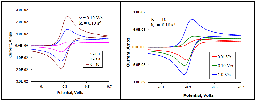
Figure 24

E_rC_iE_r Mechanism

In general, a homogeneous reaction sandwiched between two electron transfers defines an ECE mechanism. As one might imagine, the addition of a second electron transfer step leads to a good deal more complexity than in previous cases. The simplest system will be considered first – one in which a reversible electron transfer occurring at E⁰₁ is followed by an irreversible chemical step to form an electroactive product (A) whose reversible electron transfer occurs at a value for E⁰₂ that is more negative (for a reduction) than E⁰₁.

\(\begin{align}
&\mathbf{E_r}\textrm{: }\ce{Ox + ne- \Leftrightarrow Red &&E^0_1}\\
&\mathbf{C_i}\textrm{: }\mathrm{Red \xrightarrow{k_c} A} &&\\
&\mathbf{E_r}\textrm{: }\ce{A + ne- \Leftrightarrow B &&E^0_2 > E^0_1}
\end{align}\)

If on the forward scan, the potential is reversed well before the potential where A begins to reduce, the behavior of the system will mimic that of the E_rC_i case, with the peak current ratio (i_p,r / i_p,f) dependent upon the value of k_c relative to the scan rate ν. If on the other hand, one continued the potential scan through the region containing E⁰₂, the reduction of A would be observed for those conditions in which sufficient time passed to allow the product to form.

The magnitude of the current observed for the reduction of the homogenous product A is dependent upon the size of k_c and on the scan rate ν. For large k_c/slow ν, the cathodic current for this reduction will be close to that observed for the initial reduction of Ox (given similar values for n and D). On the return scan, as B in the diffusion layer is oxidized back to A, anodic current enhancements may be observed that result from the continued production of A from Red during the entire time period in which the potential is greater than E⁰₁. The oxidation peak for Red \(\rightarrow\) Ox + ne^- may not be present at longer times and larger values of k_c. Figure 25 illustrates the effect of increasing k_c at a single scan rate in the E_rC_iE_r mechanism in which the reduction potential E⁰₂ is more negative than E⁰₁. (DigiElch simulation parameters: v = 0.10 V/s; A = 0.10 cm²; C_i = 1.0 mol/cm³; D = 1.0 x 10^-5 cm²/s; α = 0.50; k_s = 100 cm/s; large K_eq; k_c = 0.01 - 10 s^-1)

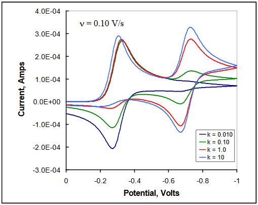
Figure 25

Now consider a system in which the reduction of the electrode product A occurs at a potential significantly (> 180 mV) more positive than the reduction of Ox.

\(\begin{align}
&\mathbf{E_r}\textrm{: }\ce{Ox + ne- \Leftrightarrow Red &&E^0_1}\\
&\mathbf{C_i}\textrm{: }\mathrm{Red \xrightarrow{k_c} A} &&\\
&\mathbf{E_r}\textrm{: }\ce{A + ne- \Leftrightarrow B &&E^0_2 < E^0_1}
\end{align}\)

In this mechanism, any A that is produced during the chemical step following the reduction of Ox will immediately be reduced to B. The observed cathodic peak will be larger than that observed for the reversible reduction of Ox alone, and will increase with increasing k_c or decreasing ν. On the return scan, the size of the anodic peak corresponding to the oxidation of Red to Ox, will be diminished in proportion to the amount of A formed during the forward scan. As the E⁰ values for the two electron transfers are well separated from each other, the oxidation of B to A will be observed following that of Red \(\rightarrow\) Ox, with the magnitude of the anodic peak also increasing with increasing k_c or decreasing ν. This mechanism is illustrated in Figure 26 for increasing values of scan rate at a fixed value of k_c. (DigiElch simulation parameters: v = 0.10 – 2.0 V/s; A = 0.10 cm²; C_i = 1.0 mol/cm³; D = 1.0 x 10^-5 cm²/s; α = 0.50; k_s = 100 cm/s; large K_eq; k_c = 1.0 s^-1)

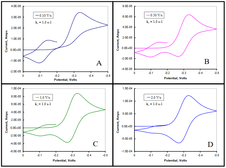
Figure 26

One of the strengths of the CV technique in the identification of electrode mechanisms is that we need not restrict ourselves to single scans that are initiated and completed at the same potential. For example, for the ECE case illustrated in Figure 26, we chose to continue the scan past the initial point, and scanned back in the cathodic direction to a potential that was negative of E⁰₂. This allowed the cathodic feature of the product electrochemical couple (A/B) to be observed. By controlling the initial, switching, and final potentials, along with the number of scans, more complicated mechanisms can be probed. Imagine what you might see if the product of the homogeneous reaction following electron transfer to Ox itself underwent homogeneous reaction to form an electrochemically active product. Can you say ECECE?

Detailed treatment of electrode mechanisms is beyond the scope of this module. Supporting theoretical discussions for the cases presented here as well as less common and more complicated mechanisms are available in cited references for the interested reader.^10-13