a) Linear Sweep Voltammetry

In a previous section, we presented the diffusion controlled current-time behavior of a redox couple following a step to a potential sufficient to reduce all of the electroactive species near the surface of the electrode. Faradaic current was observed to decay as a function of t^-1/2 according to the Cottrell equation. This was explained in terms of the concentration profile extending from the electrode surface into the bulk of solution. The thickness of this diffusion layer increases with time, decreasing the slope of the concentration gradient, and thus reducing the observed current.

We must now consider what happens to the concentration of electroactive species near the electrode as the potential is scanned, rather than stepped. Instead of going immediately to zero, the concentration of Ox is now dependent on the magnitude of the applied potential with respect to the E⁰’, with the ratio of C_Red to C_Ox (at 25 ^oC) given by the Nernst equation

\[\mathrm{E = E^0}\mathrm{’– (0.059 / n) \log [C_{Red}/ C_{Ox}]}\]

For our discussion, it is convenient to express the applied potential, E, in terms of its proximity to E⁰’, rearranging the Nernst equation as follows

\[\mathrm{\dfrac{n({E^0}'−E)}{0.059}=\log\dfrac{C_{Red}}{C_{Ox}}}\]

The concentration gradients existing for Ox and Red at several values of [n (E⁰' − E)] are illustrated in Figure 15 (0.059 V = 59 mV).

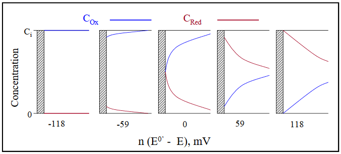
Figure 15

For a 1-electron reduction under diffusion control with an applied potential 118 mV positive of the E⁰’, C_Ox = 100 C_Red at the electrode surface. A potential 59 mV positive of the E⁰’ yields C_Ox = 10 C_Red. When the applied potential equals the E⁰’, (E⁰' − E) = 0, and the two concentrations are equal adjacent to the electrode, with each being half of the initial, or bulk concentration of C_Ox (C_i in Figure 15). Beyond the E⁰’, the concentration of C_Red becomes larger than that of C_Ox, with C_Red = 10 C_Ox at a point 59 mV more negative than the E⁰’, and 100 C_Ox at a point 118 mV more negative.

An important difference in the concentration gradients for potential sweep experiments when compared to large potential step experiments is that the slope of the gradient is dependent upon both the C_Ox at the electrode surface (non-zero in the vicinity of E⁰’) and the thickness of the diffusion layer, not just the latter. A consequence of this is that the maximum concentration gradient (and hence maximum current) is observed at a potential 28.5 mV (for n = 1) beyond the E⁰’ of the redox couple. The potential – time and current – potential curves are presented in Figure 16 for a 1-electron, diffusion controlled redox couple with an E⁰’ of -0.300 V. The rate at which the potential is scanned is called the scan rate (big surprise) and is represented by v, generally with units of V/s. The initial potential is 0.00 V, with the final potential equal to -0.50 V. The current decrease beyond the peak potential (-0.328 V) is the result of C_Ox at the electrode surface being driven to zero and the extension of the diffusion layer further and further into solution as the scan continues. (DigiElch simulation parameters: v = 0.100 V/s; A = 0.050 cm²; C_i = 1.0 mol/cm³; D = 1.0 x 10^-5 cm²/s; α = 0.50; k_s = 100 cm/s)

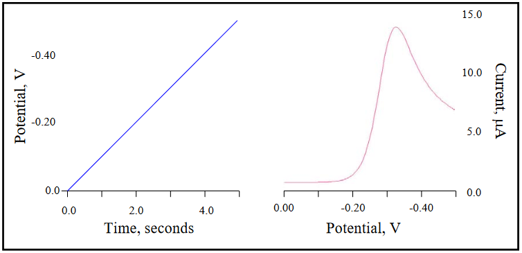
Figure 16

The observed peak current, i_p, for a reversible electron transfer in LSV is given by the Randles-Sevcik equation

\[\mathrm{i_p = (2.69 \times 10^5)\, n^{3/2}\, A\, D^{1/2}\, C_i\,} v^{1/2}\]

where 2.69 x 10^-5 is a collection of constants at 25 ^oC, and the variables are as previously defined. The capacitive current, which appears as the non-zero baseline at the left of the current-potential scan, must be subtracted from the total current to correctly obtain i_p. Most commercial instrumentation allows for this to be done digitally.

LSV can be used to determine such parameters for a reversible system as E⁰’ , n, D, and C_i, while the use of a known redox couple can be employed in the calculation of A. As we have seen, the E⁰’ value occurs at a point (28.5/n) mV positive (for a reduction) of the observed peak potential, E_p. If difficulty is experienced with the accurate location of a peak potential, the potential measured at half the peak height (E_p/2) can be used to calculate it, lying (56.5/n) mV more positive than the E_p (for a reduction). If a value for D is known, the n-value for a redox active species can be calculated using the Randles-Sevcik equation. In most cases, even D values estimated from similar structures with known diffusion coefficients will suffice.

A plot of peak current, i_p, as a function of v^1/2, is linear for a redox active species under diffusion control, and can be a useful diagnostic indicator for a redox system being characterized for the first time. For reversible electron transfer, the position of E_p will not change with scan rate. The separation between E_1/2 and E_p can also be used to diagnose reversible electron transfer, with |E_p – E_p/2| equal to (56.5/n) mV for a reversible electron transfer (k_s > 0.02 cm/s). For irreversible electron transfer (k_s < 5 x 10^-5 cm/s), |E_p – E_p/2| will equal (47.7/αn) mV. Intermediate values for k_s, defining the quasi-reversible regime, will yield intermediate values for |E_p – E_p/2| as well.