15.2: Förster Resonance Energy Transfer (FRET)

Förster resonance energy transfer (FRET) refers to the nonradiative transfer of an electronic excitation from a donor molecule to an acceptor molecule:

\[\ce{D}^{*} + \ce{A} \rightarrow \ce{D} + \ce{A}^{*} \label{14.1}\]

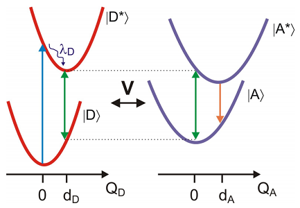
This electronic excitation transfer, whose practical description was first given by Förster, arises from a dipole–dipole interaction between the electronic states of the donor and the acceptor, and does not involve the emission and reabsorption of a light field. Transfer occurs when the oscillations of an optically induced electronic coherence on the donor are resonant with the electronic energy gap of the acceptor. The strength of the interaction depends on the magnitude of a transition dipole interaction, which depends on the magnitude of the donor and acceptor transition matrix elements, and the alignment and separation of the dipoles. The sharp \(1/r^6\) dependence on distance is often used in spectroscopic characterization of the proximity of donor and acceptor.

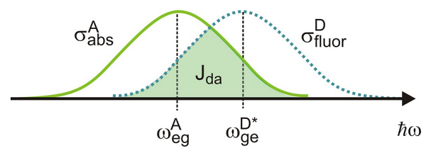
The electronic ground and excited states of the donor and acceptor molecules all play a role in FRET. We consider the case in which we have excited the donor electronic transition, and the acceptor is in the ground state. Absorption of light by the donor at the equilibrium energy gap is followed by rapid vibrational relaxation that dissipates the reorganization energy of the donor \(\lambda _ {D}\) over the course of picoseconds. This leaves the donor in a coherence that oscillates at the energy gap in the donor excited state \(\omega _ {e g}^{D} \left( q _ {D} = d _ {D} \right)\). The time scale for FRET is typically nanoseconds, so this preparation step is typically much faster than the transfer phase. For resonance energy transfer we require a resonance condition, so that the oscillation of the excited donor coherence is resonant with the ground state electronic energy gap of the acceptor \(\omega _ {e g}^{A} \left( q _ {A} = 0 \right)\). Transfer of energy to the acceptor leads to vibrational relaxation and subsequent acceptor fluorescence that is spectrally shifted from the donor fluorescence. In practice, the efficiency of energy transfer is obtained by comparing the fluorescence emitted from donor and acceptor.

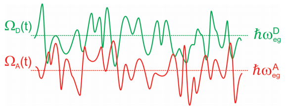
This description of the problem lends itself naturally to treating with a DHO Hamiltonian, However, an alternate picture is also applicable, which can be described through the EG Hamiltonian. FRET arises from the resonance that occurs when the fluctuating electronic energy gap of a donor in its excited state matches the energy gap of an acceptor in its ground state. In other words

\[\underbrace {\hbar \omega _ {e g}^{D} - \lambda _ {D}} _ {\Omega _ {D} (t)} = \underbrace {\hbar \omega _ {e g}^{A} - \lambda _ {A}} _ {\Omega _ {A} (t)} \label{14.2}\]

These energy gaps are time-dependent with occasion crossings that allow transfer of energy.

Our system includes the ground and excited potentials of the donor and acceptor molecules. The four possible electronic configurations of the system are

\[| G _ {D} G _ {A} \rangle , | E _ {D} G _ {A} \rangle , | G _ {D} E _ {A} \rangle , | E _ {D} E _ {A} \rangle\]

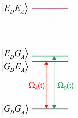
Here the notation refers to the ground (\(G\)) or excited (\(E\)) vibronic states of either donor (\(D\)) or acceptor (\(A\)). More explicitly, the states also include the vibrational excitation:

\[| E _ {D} G _ {A} \rangle = | e _ {D} n _ {D} ; g _ {A} n _ {A} \rangle\]

Thus the system can have no excitation, one excitation on the donor, one excitation on the acceptor, or one excitation on both donor and acceptor. For our purposes, let’s only consider the two electronic configurations that are close in energy, and are likely to play a role in the resonance transfer in Equation \ref{14.2} and

\(| E _ {D} G _ {A} \rangle\) and \(| G _ {D} E _ {A} \rangle\)

Since the donor and acceptor are weakly coupled, we can write our Hamiltonian for this problem in a form that can be solved by perturbation theory (\(H = H _ {0} + V\)). Working with the DHO. approach, our material Hamiltonian has four electronic manifolds to consider:

\[\underbrace {\hbar \omega _ {e g}^{D} - \lambda _ {D}} _ {\Omega _ {D} (t)} = \underbrace {\hbar \omega _ {e g}^{A} - \lambda _ {A}} _ {\Omega _ {A} (t)} \label{14.3}\]

Each of these is defined as we did previously, with an electronic energy and a dependence on a displaced nuclear coordinate. For instance

\[\begin{align} H _ {D}^{E} &= | e _ {D} \rangle E _ {e}^{D} \langle e _ {D} | + H _ {e}^{D} \label{14.4} \\[4pt] H _ {e}^{D} &= \hbar \omega _ {0}^{D} \left( \tilde {p} _ {D}^{2} + \left( \tilde {q} _ {D} - \tilde {d} _ {D} \right)^{2} \right) \label{14.5} \end{align}\]

\(E _ {e}^{D}\) is the electronic energy of donor excited state.

Then, what is \(V\)? Classically it is a Coulomb interaction of the form ,

\[V = \sum _ {i j} \frac {q _ {i}^{D} q _ {j}^{A}} {\left| r _ {i}^{D} - r _ {j}^{A} \right|} \label{14.6}\]

Here the sum is over all electrons and nuclei of the donor (\(i\)) and acceptor (\(j\)).

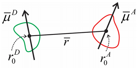
As is, this is challenging to work with, but at large separation between molecules, we can recast this as a dipole–dipole interaction. We define a frame of reference for the donor and acceptor molecule, and assume that the distance between molecules is large. Then the dipole moments for the molecules are

\[\begin{aligned} \overline {\mu}^{D} & = \sum _ {i} q _ {i}^{D} \left( r _ {i}^{D} - r _ {0}^{D} \right) \\ \overline {\mu}^{A} & = \sum _ {j} q _ {j}^{A} \left( r _ {J}^{A} - r _ {0}^{A} \right) \end{aligned} \label{14.7}\]

The interaction between donor and acceptor takes the form of a dipole–dipole interaction:

\[V = \dfrac {3 \left( \overline {\mu} _ {A} \cdot \hat {r} \right) \left( \overline {\mu} _ {D} \cdot \hat {r} \right) - \overline {\mu} _ {A} \cdot \overline {\mu} _ {D}} {\overline {r}^{3}} \label{14.8}\]

where \(r\) is the distance between donor and acceptor dipoles and \(\hat{r}\) is a unit vector that marks the direction between them. The dipole operators here are taken to only act on the electronic states and be independent of nuclear configuration, i.e., the Condon approximation. We write the transition dipole matrix elements that couple the ground and excited electronic states for the donor and acceptor as

\[ \begin{align} \overline {\mu} _ {A} &= | A \rangle \overline {\mu}_{AA^{*}} \left\langle A^{*} | + | A^{*} \right\rangle \overline {\mu} _ {A^{*} A} \langle A | \label{14.9} \\[4pt] \overline {\mu} _ {D} &= | D \rangle \overline {\mu} _ {D D^{*}} \left\langle D^{*} | + | D^{*} \right\rangle \overline {\mu} _ {D^{*} D} \langle D | \label{14.10} \end{align} \]

For the dipole operator, we can separate the scalar and orientational contributions as

\[\overline {\mu} _ {A} = \hat {u} _ {A} \mu _ {A} \label{14.11}\]

This allows the transition dipole interaction in Equation \ref{14.8} to be written as

\[V = \mu _ {A} \mu _ {B} \frac {\kappa} {r^{3}} [ | D^{*} A \rangle \left\langle A^{*} D | + | A^{*} D \right\rangle \left\langle D^{*} A | \right] \label{14.12}\]

All of the orientational factors are now in the term \(\kappa\)

\[\kappa = 3 \left( \hat {u} _ {A} \cdot \hat {r} \right) \left( \hat {u} _ {D} \cdot \hat {r} \right) - \hat {u} _ {A} \cdot \hat {u} _ {D} \label{14.13}\]

We can now obtain the rates of energy transfer using Fermi’s Golden Rule expressed as a correlation function in the interaction Hamiltonian:

\[w _ {k \ell} = \frac {2 \pi} {\hbar^{2}} \sum _ {\ell} p _ {\ell} \left| V _ {k \ell} \right|^{2} \delta \left( \omega _ {k} - \omega _ {\ell} \right) = \frac {1} {\hbar^{2}} \int _ {- \infty}^{+ \infty} d t \left\langle V _ {I} (t) V _ {I} ( 0 ) \right\rangle \label{14.14}\]

Note that this is not a Fourier transform! Since we are using a correlation function there is an assumption that we have an equilibrium system, even though we are initially in the excited donor state. This is reasonable for the case that there is a clear time scale separation between the ps vibrational relaxation and thermalization in the donor excited state and the time scale (or inverse rate) of the energy transfer process.

Now substituting the initial state \(\ell = | D^{*} A \rangle\) and the final state \(k = | A^{*} D \rangle\), we find

\[w _ {E T} = \frac {1} {\hbar^{2}} \int _ {- \infty}^{+ \infty} d t \frac {\left\langle \kappa^{2} \right\rangle} {r^{6}} \left\langle D^{*} A \left| \mu _ {D} (t) \mu _ {A} (t) \mu _ {D} ( 0 ) \mu _ {A} ( 0 ) \right| D^{*} A \right\rangle \label{14.15}\]

where

\[\mu _ {D} (t) = e^{i H _ {D} t / \hbar} \mu _ {D} e^{- i H _ {D} t / \hbar}.\]

Here, we have neglected the rotational motion of the dipoles. Most generally, the orientational average is

\[\left\langle \kappa^{2} \right\rangle = \langle \kappa (t) \kappa ( 0 ) \rangle \label{14.16}\]

However, this factor is easier to evaluate if the dipoles are static, or if they rapidly rotate to become isotropically distributed. For the static case \(\left\langle \kappa^{2} \right\rangle = 0.475\). For the case of fast loss of orientation:

\[\left\langle \kappa^{2} \right\rangle \rightarrow \langle \kappa (t) \rangle \langle \kappa ( 0 ) \rangle = \langle \kappa \rangle^{2} = \dfrac{2}{3}\]

Since the dipole operators act only on \(A\) or \(D^{*}\), and the \(D\) and \(A\) nuclear coordinates are orthogonal, we can separate terms in the donor and acceptor states.

\[\begin{aligned} w _ {E T} & = \frac {1} {\hbar^{2}} \int _ {- \infty}^{+ \infty} d t \frac {\left\langle \kappa^{2} \right\rangle} {r^{6}} \left\langle D^{*} \left| \mu _ {D} (t) \mu _ {D} ( 0 ) \right| D^{*} \right\rangle \left\langle A \left| \mu _ {A} (t) \mu _ {A} ( 0 ) \right| A \right\rangle \\ & = \frac {1} {\hbar^{2}} \int _ {- \infty}^{+ \infty} d t \frac {\left\langle \kappa^{2} \right\rangle} {r^{6}} C _ {D^{*} D^{*}} (t) C _ {\mathrm {AA}} (t) \end{aligned} \label{14.17}\]

The terms in this equation represent the dipole correlation function for the donor initiating in the excited state and the acceptor correlation function initiating in the ground state. That is, these are correlation functions for the donor emission (fluorescence) and acceptor absorption. Remembering that \(| D^{*} \rangle\) represents the electronic and nuclear configuration \(| d^{*} n _ {D^{*}} \rangle\), we can use the displaced harmonic oscillator Hamiltonian or energy gap Hamiltonian to evaluate the correlation functions. For the case of Gaussian statistics we can write

\[C _ {D _ {D}^{*}} \cdot (t) = \left| \mu _ {D D^{*}} \right|^{2} e^{- i \left( \omega _ {D D^{*}} - 2 \lambda _ {D} \right) t^{*} - g _ {D}^{*} (t)} \label{14.18}\]

\[C _ {A A} (t) = \left| \mu _ {A A} \right|^{2} e^{- i \omega _ {A A} t - g _ {A} (t)} \label{14.19}\]

Here we made use of

\[ \omega _ {D^{*} D} = \omega _ {D D^{*}} - 2 \lambda _ {D}\label{14.20}\]

which expresses the emission frequency as a frequency shift of \(2 \lambda _ {D}\) relative to the donor absorption frequency. The dipole correlation functions can be expressed in terms of the inverse Fourier transforms of a fluorescence or absorption lineshape:

\[C _ {D^{*} D^{\cdot}} (t) = \frac {1} {2 \pi} \int _ {- \infty}^{+ \infty} d \omega e^{- i \omega t} \sigma _ {f l u o r}^{D} ( \omega ) \label{14.21}\]

\[C _ {A A} (t) = \frac {1} {2 \pi} \int _ {- \infty}^{+ \infty} d \omega e^{- i \omega t} \sigma _ {a b s}^{A} ( \omega ) \label{14.22}\]

To express the rate of energy transfer in terms of its common practical form, we make use of Parsival’s Theorem, which states that if a Fourier transform pair is defined for two functions, the integral over a product of those functions is equal whether evaluated in the time or frequency domain:

\[\int _ {- \infty}^{\infty} f _ {1} (t) f _ {2}^{*} (t) d t = \int _ {- \infty}^{\infty} \tilde {f} _ {1} ( \omega ) \tilde {f} _ {2}^{*} ( \omega ) d \omega \label{14.23}\]

This allows us to express the energy transfer rate as an overlap integral \(J_{DA}\) between the donor fluorescence and acceptor absorption spectra:

\[w _ {E T} = \frac {1} {\hbar^{2}} \frac {\left\langle \kappa^{2} \right\rangle} {r^{6}} \left| \mu _ {D D^{*}} \right|^{2} \left| \mu _ {A A^{\prime}} \right|^{2} \int _ {- \infty}^{+ \infty} d \omega \sigma _ {a b s}^{A} ( \omega ) \sigma _ {f u o r}^{D} ( \omega ) \label{14.24}\]

Here   is the lineshape normalized to the transition matrix element squared: \(\sigma = \sigma / | \mu |^{2}\). The overlap integral is a measure of resonance between donor and acceptor transitions.

So, the energy transfer rate scales as \(r^{-6}\), depends on the strengths of the electronic transitions for donor and acceptor molecules, and requires resonance between donor fluorescence and acceptor absorption. One of the things we have neglected is that the rate of energy transfer will also depend on the rate of excited donor state population relaxation. Since this relaxation is typically dominated by the donor fluorescence rate, the rate of energy transfer is commonly written in terms of an effective distance \(R_0\), and the fluorescence lifetime of the donor \(\tau_D\):

\[w _ {E T} = \frac {1} {\tau _ {D}} \left( \frac {R _ {0}} {r} \right)^{6} \label{14.25}\]

At the critical transfer distance \(R_0\) the rate (or probability) of energy transfer is equal to the rate of fluorescence. \(R_0\) is defined in terms of the sixth-root of the terms in Equation \ref{14.24}, and is commonly written as

\[R _ {0}^{6} = \frac {9000 \ln ( 10 ) \phi _ {D} \left\langle \kappa^{2} \right\rangle} {128 \pi^{5} n^{4} N _ {A}} \int _ {0}^{\infty} d \overline {\nu} \frac {\sigma _ {\text {fluur}}^{D} ( \overline {V} ) \varepsilon _ {A} ( \overline {v} )} {\overline {V}^{4}} \label{14.26}\]

This is the practical definition that accounts for the frequency dependence of the transitiondipole interaction and non-radiative donor relaxation in addition to being expressed in common units. \(\overline {V}\) represents units of frequency in cm^-1. The fluorescence spectrum \(\sigma_{\text {fluor}}^{D}\) must be normalized to unit area, so that at \(\sigma_{\text {fluor }}^{D}(\bar{v})\) is expressed in cm (inverse wavenumbers). The absorption spectrum \(\varepsilon_{A}(\bar{v})\) must be expressed in molar decadic extinction coefficient units (liter/mol*cm). \(n\) is the index of refraction of the solvent, \(N_A\) is Avagadro’s number, and \(\phi_D\) is the donor fluorescence quantum yield.

Transition Dipole Interaction

FRET is one example of a quantum mechanical transition dipole interaction. The interaction between two dipoles, \(A\) and \(D\), in Equation \ref{14.12} is

\[V = \frac {\kappa} {r^{3}} \left\langle e \left| \mu _ {A} \right| g \right\rangle \left\langle g \left| \mu _ {D} \right| e \right\rangle \label{14.27}\]

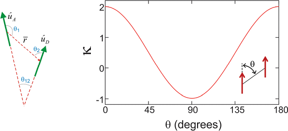
Here, \(\left\langle g \left| \mu _ {D} \right| e \right\rangle\) is the transition dipole moment in Debye for the ground-to-excited state transition of molecule \(A\). \(r\) is the distance between the centers of the point dipoles, and \(\kappa\) is the unitless orientational factor

\[\kappa = 3 \cos \theta _ {1} \cos \theta _ {2} - \cos \theta _ {12}\]

The figure below illustrates this function for the case of two parallel dipoles, as a function of the angle between the dipole and the vector defining their separation.

In the case of vibrational coupling, the dipole operator is expanded in the vibrational normal coordinate: \(\mu = \mu _ {0} + \left( \partial \mu / \partial Q _ {A} \right) Q _ {A}\) and harmonic transition dipole matrix elements are

\[\left\langle 1\left|\mu_{A}\right| 0\right\rangle=\sqrt{\frac{\hbar}{2 c \omega_{A}}} \frac{\partial \mu}{\partial Q_{A}} \label{14.28}\]

where \(\omega _ {A}\) is the vibrational frequency. If the frequency \(V _ {A}\) is given in cm^-1, and the transition dipole moment \(\partial \mu / \partial Q _ {A}\) is given in units of \(\begin{equation}\text { D } Å^{-1} \text {amu }^{-1 / 2}\end{equation}\), then the matrix element in units of \(D\) is

\[\left| \left\langle 1 \left| \mu _ {A} \right| 0 \right\rangle \right| = 4.1058 v _ {A}^{- 1 / 2} \left( \partial \mu / \partial Q _ {A} \right)\]

If the distance between dipoles is specified in Ångstroms, then the transition dipole coupling from Equation \ref{14.27} in cm^-1 is

\[V \left( c m^{- 1} \right) = 5034 \kappa r^{- 3}.\]

Experimentally, one can determine the transition dipole moment from the absorbance \(A\) as

\[A = \left( \frac {\pi N _ {A}} {3 c^{2}} \right) \left( \frac {\partial \mu} {\partial Q _ {A}} \right)^{2} \label{14.29}\]

Readings

1. Cheam, T. C.; Krimm, S., Transition dipole interaction in polypeptides: Ab initio calculation of transition dipole parameters. Chemical Physics Letters 1984, 107, 613-616.
2. Forster, T., Transfer mechanisms of electronic excitation. Discussions of the Faraday Society 1959, 27, 7-17.
3. Förster, T., Zwischenmolekulare Energiewanderung und Fluoreszenz. Annalen der Physik 1948, 437, 55-75.
4. Förster, T., Experimentelle und theoretische Untersuchung des zwischenmolecularen Uebergangs von Electronenanregungsenergie. Z. Naturforsch 1949, 4A, 321–327