14.4: The Energy Gap Hamiltonian

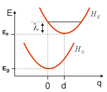
In describing fluctuations in a quantum mechanical system, we describe how an experimental observable is influenced by its interactions with a thermally agitated environment. For this, we work with the specific example of an electronic absorption spectrum and return to the Displaced Harmonic Oscillator (DHO) model. We previously described this model in terms of the eigenstates of the material Hamiltonian \(H_0\), and interpreted the dipole correlation function and resulting lineshape in terms of the overlap between two wave packets evolving on the ground and excited surfaces \(| E \rangle\) and \(| G \rangle\).

\[C _ {\mu \mu} (t) = \left| \mu _ {e g} \right|^{2} e^{- i \left( E _ {e} - E _ {g} \right) t / \hbar} \left\langle \varphi _ {g} (t) | \varphi _ {e} (t) \right\rangle \label{13.43}\]

It is worth noting a similarity between the DHO Hamiltonian, and a general form for the interaction of an electronic two-level “system” with a harmonic oscillator “bath” whose degrees of freedom are dark to the observation, but which influence the behavior of the system.

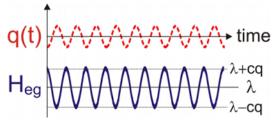
Expressed in a slightly different physical picture, we can also conceive of this process as nuclear motions that act to modulate the electronic energy gap \(\omega _ {e g}\). We can imagine rewriting the same Hamiltonian in a form with a new physical picture that desscribes the electronic energy gap’s dependence on \(q\), i.e., its variation relative to \(\omega _ {e g}\). If we define an Energy Gap Hamiltonian:

\[H _ {e g} = H _ {e} - H _ {g}\]

we can rewrite the DHO Hamiltonian

\[H _ {0} = | e \rangle E _ {e} \langle e | + | g \rangle E _ {g} \langle g | + H _ {e} + H _ {g} \label{13.44}\]

as an electronic transition linearly coupled to a harmonic oscillator:

\[H _ {0} = | e \rangle E _ {e} \langle e | + | g \rangle E _ {g} \langle g | + H _ {e g} + 2 H _ {g} \label{13.44B}\]

Noting that

\[H _ {g} = \frac {p^{2}} {2 m} + \frac {1} {2} m \omega _ {0}^{2} q^{2} \label{13.44C}\]

we can write this as a system-bath Hamiltonian:

\[H _ {0} = H _ {S} + H _ {B} + H _ {S B} \label{13.44D}\]

where \(H_{SB}\) describes the interaction of the electronic system (\(H_S\)) with the vibrational bath (\(H_B\)). Here

\[H _ {S} = | e \rangle E _ {e} \langle e | + | g \rangle E _ {g} \langle g |\]

\[H _ {B} = 2 H _ {g}\]

and

\[\begin{align} H _ {S B} = H _ {e g} &= \dfrac {1} {2} m \omega _ {0}^{2} ( q - d )^{2} - \frac {1} {2} m \omega _ {0}^{2} q^{2} \\ &= - m \omega _ {0}^{2} d q + \frac {1} {2} m \omega _ {0}^{2} d^{2} \\ &= - c q + \lambda \end{align}\]

The Energy Gap Hamiltonian describes a linear coupling between the electronic transition and a harmonic oscillator. The strength of the coupling is \(c\) and the Hamiltonian has a constant energy offset value given by the reorganization energy (\(\lambda\)). Any motion in the bath coordinate \(q\) introduces a proportional change in the electronic energy gap.

In an alternate form, the Energy Gap Hamiltonian can also be written to incorporate the reorganization energy into the system:

\[\begin{align*} H _ {0} &= | e \rangle E _ {e} \langle e | + | g \rangle E _ {g} \langle g | + H _ {e g} + 2 H _ {g} \label{13.44E} \\[4pt] H _ {S}^{\prime} &= | e \rangle \left( E _ {e} + \lambda \right) \langle e | + | g \rangle E _ {g} \langle g | \\[4pt] H _ {B}^{\prime} &= \frac {p^{2}} {2 m} + \frac {1} {2} m \omega _ {0}^{2} q^{2} \\[4pt] H _ {S B}^{\prime} &= - m \omega _ {0}^{2} d q \end{align*}\]

This formulation describes fluctuations about the average value of the energy gap \(\hbar \omega _ {e g} + \lambda\), however, the observables calculated are the same.

From the picture of a modulated energy gap one can begin to see how random fluctuations can be treated by coupling to a harmonic bath. If each oscillator modulates the energy gap at a given frequency, and the phase between oscillators is random as a result of their independence, then time-domain fluctuations and dephasing can be cast in terms of a Fourier spectrum of couplings to oscillators with continuously varying frequency.

Energy Gap Hamiltonian

Now let’s work through the description of electronic spectroscopy with the Energy Gap Hamiltonian more carefully. Working from Equations \ref{13.43} and \ref{13.44} we express the energy gap Hamiltonian through reduced coordinates for the momentum, coordinate, and displacement of the oscillator.

\[p = \hat {p} \left( 2 \hbar \omega _ {0} m \right)^{- 1 / 2}\]

\[q = \hat {q} \left( m \omega _ {0} / 2 \hbar \right)^{1 / 2}\]

\[d = d \left( m \omega _ {0} / 2 \hbar \right)^{1 / 2}\]

with

\[ \begin{align} H _ {e} &= \hbar \omega _ {0} \left( p^{2} + ( q - d )^{2} \right) \\[4pt] H_{g} &= \hbar \omega _ {0} \left( p^{2} + q^{2} \right) \end{align} \label{13.48}\]

From Equation \ref{13.43} we have

\[\left.\begin{aligned} H _ {e g} & = - 2 \hbar \omega _ {0} d q + \hbar \omega _ {0} d^{2} \\ & = - m \omega _ {0}^{2} d q + \lambda \end{aligned} \right. \label{13.49}\]

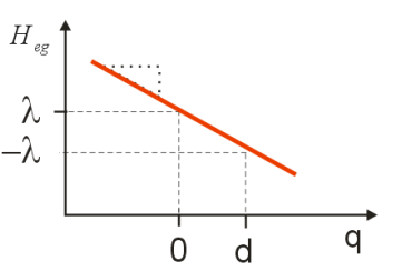
The energy gap Hamiltonian describes a linear coupling of the electronic system to the coordinate q. The slope of \(H_{eg}\) versus \(q\) is the coupling strength, and the average value of \(H_{eg}\) in the ground state, \(H _ {e g} ( q = 0 )\), is offset by the reorganization energy \(\lambda\). We note that the average value of the energy gap Hamiltonian is \(\left\langle H _ {e g} \right\rangle = \lambda\).

To obtain the absorption lineshape from the dipole correlation function

\[C _ {\mu \mu} (t) = \left| \mu _ {e g} \right|^{2} e^{- i \omega _ {e g} t} F (t) \label{13.50}\]

we must evaluate the dephasing function.

\[F (t) = \left\langle e^{i H _ {g} t} e^{- i H _ {e} t} \right\rangle = \left\langle U _ {g}^{\dagger} U _ {e} \right\rangle \label{13.51}\]

We want to rewrite the dephasing function in terms of the time dependence to the energy gap \(H_{eg}\); that is, if \(F (t) = \left\langle U _ {c g} \right\rangle\), then what is \(U _ {e g}\)? This involves a unitary transformation of the dynamics to a new frame of reference. The transformation from the DHO Hamiltonian to the EG Hamiltonian is similar to our derivation of the interaction picture.

Transformation of time-propagators

If we have a time dependent quantity of the form

\[e^{i H _ {A} t} A e^{- i H _ {B} t} \label{13.52}\]

we can also express the dynamics through the difference Hamiltonian \(H _ {B A} = H _ {B} - H _ {A}\)

\[A e^{- i \left( H _ {B} - H _ {A} \right) t} = A e^{- i H _ {B A} t} \label{13.53}\]

using a commonly performed unitary transformation. If we write

\[H _ {B} = H _ {A} + H _ {B A} \label{13.54}\]

we can use the same procedure for partitioning the dynamics in the interaction picture to write

\[e^{- i H _ {B t} t} = e^{- i H _ {A} t} \exp _ {+} \left[ - \frac {i} {\hbar} \int _ {0}^{t} d \tau H _ {B A} ( \tau ) \right] \label{13.55}\]

where

\[H _ {B A} ( \tau ) = e^{i H _ {A} t} H _ {B A} e^{- i H _ {A} t} \label{13.56}\]

Then, we can also write:

\[e^{i H _ {A} t} e^{- i H _ {B} t} = \exp _ {+} \left[ - \frac {i} {\hbar} \int _ {0}^{t} d \tau H _ {B A} ( \tau ) \right] \label{13.57}\]

Noting the mapping to the interaction picture

\[H _ {e} = H _ {g} + H _ {e g} \quad \Leftrightarrow \quad H = H _ {0} + V \label{13.58}\]

we see that we can represent the time dependence of the electronic energy gap \(H_{eg}\) using

\[e^{- i H _ {c} t / h} = e^{- i H _ {g} t / h} \exp _ {+} \left[ \frac {- i} {\hbar} \int _ {0}^{t} d \tau H _ {e g} ( \tau ) \right] \label{13.59}\]

\[U _ {e} = U _ {g} U _ {e g}\]

where

\[\begin{align} H _ {e g} (t) & = e^{i H _ {g} t / \hbar} H _ {e g} e^{- i H _ {g} t / \hbar} \\ & = U _ {g}^{\dagger} H _ {e g} U _ {g} \label{13.60} \end{align} \]

Remembering the equivalence between the harmonic mode \(H_g\) and the bath mode(s) \(H_B\) indicates that the time dependence of the EG Hamiltonian reflects how the electronic energy gap is modulated as a result of the interactions with the bath. That is \(U _ {g} \Leftrightarrow U _ {B}\).

Equation \ref{13.59} immediately implies that

\[F (t) = \left\langle e^{i H _ {g} t / \hbar} e^{- i H _ {e} t / \hbar} \right\rangle = \left\langle \exp _ {+} \left[ \frac {- i} {\hbar} \int _ {0}^{t} d \tau H _ {e g} ( \tau ) \right] \right\rangle \label{13.61}\]

Now the quantum dephasing function is in the same form as we saw in our earlier classical derivation. Using the second-order cumulant expansion allows the dephasing function to be written as

\[F (t) = \left\langle e^{i H _ {g} t / \hbar} e^{- i H _ {e} t / \hbar} \right\rangle = \left\langle \exp _ {+} \left[ \frac {- i} {\hbar} \int _ {0}^{t} d \tau H _ {e g} ( \tau ) \right] \right\rangle \label{13.62}\]

Note that the cumulant expansion is here written as a time-ordered expansion. The first exponential term depends on the mean value of \(H_{eg}\)

\[\left\langle H _ {e g} \right\rangle = \hbar \omega _ {0} d^{2} = \lambda \label{13.63}\]

This is a result of how we defined \(H_{eg}\). Alternatively, the EG Hamiltonian could have been defined relative to the energy gap at \(Q=0\): \(H _ {e g} = H _ {e} - H _ {g} + \lambda\). In this case the leading term in Equation \ref{13.62} would be zero, and the mean energy gap that describes the high frequency (system) oscillation in the dipole correlation function is \(\omega _ {e g} + \lambda\).

The second exponential term in Equation \ref{13.62} is a correlation function that describes the time dependence of the energy gap

\[\left. \begin{array} {c} {\left\langle H _ {e g} \left( \tau _ {2} \right) H _ {e g} \left( \tau _ {1} \right) \right\rangle - \left\langle H _ {e g} \left( \tau _ {2} \right) \right\rangle \left\langle H _ {e g} \left( \tau _ {1} \right) \right\rangle} \\ {= \left\langle \delta H _ {e g} \left( \tau _ {2} \right) \delta H _ {e g} \left( \tau _ {1} \right) \right\rangle} \end{array} \right. \label{13.64}\]

where

\[\left.\begin{aligned} \delta H _ {e g} & = H _ {e g} - \left\langle H _ {e g} \right\rangle \\ & = - m \omega _ {0}^{2} d q \end{aligned} \right. \label{13.65}\]

Defining the time-dependent energy gap transition frequency in terms of the EG Hamiltonian as

\[\delta \hat {\omega} _ {e g} \equiv \frac {\delta H _ {e g}} {\hbar} \label{13.66}\]

we can write the energy gap correlation function

\[C _ {e g} \left( \tau _ {2} , \tau _ {1} \right) = \left\langle \delta \hat {\omega} _ {e g} \left( \tau _ {2} - \tau _ {1} \right) \delta \hat {\omega} _ {e g} ( 0 ) \right\rangle \label{13.68}\]

It follows that

\[F (t) = e^{- i \lambda t / \hbar} e^{- g (t)}\]

and

\[g (t) = \int _ {0}^{t} d \tau _ {2} \int _ {0}^{\tau _ {2}} d \tau _ {1} C _ {e g} \left( \tau _ {2} , \tau _ {1} \right) \label{13.69}\]

and the dipole correlation function can be expressed as

\[C _ {\mu \mu} (t) = \left| \mu _ {e g} \right|^{2} e^{- i \left( E _ {e} - E _ {g} + \lambda \right) t / \hbar} e^{- g (t)} \label{13.70}\]

This is the correlation function expression that determines the absorption lineshape for a timedependent energy gap. It is a general expression at this point, for all forms of the energy gap correlation function. The only approximation made for the bath is the second cumulant expansion.

Now, let’s look specifically at the case where the bath we are coupled to is a single harmonic mode. The energy gap correlation function is evaluated from

\[\left.\begin{aligned} C _ {e g} (t) & = \sum _ {n} p _ {n} \left\langle n \left| \delta \hat {\omega} _ {e g} (t) \delta \hat {\omega} _ {e g} ( 0 ) \right| n \right\rangle \\ & = \frac {1} {\hbar^{2}} \sum _ {n} p _ {n} \left\langle n \left| e^{i H _ {g} t / \hbar} \delta H _ {e g} e^{- i H _ {g} t / \hbar} \delta H _ {e g} \right| n \right\rangle \end{aligned} \right. \label{13.71}\]

Noting that the bath oscillator correlation function

\[C _ {q q} (t) = \langle q (t) q ( 0 ) \rangle = \frac {\hbar} {2 m \omega _ {0}} \left[ ( \overline {n} + 1 ) e^{- i \omega _ {0} t} + \overline {n} e^{i \omega _ {0} t} \right] \label{13.72}\]

we find

\[C _ {e g} (t) = \omega _ {0}^{2} D \left[ ( \overline {n} + 1 ) e^{- i \omega _ {0} t} + \overline {n} e^{i \omega _ {0} t} \right] \label{13.73}\]

Here, as before, \(\beta = 1 / k _ {B} T\), \(\overline {n}\) is the thermally averaged occupation number for the oscillator

\[\overline {n} = \sum _ {n} p _ {n} \left\langle n \left| a^{\dagger} a \right| n \right\rangle = \left( e^{\beta \hbar \omega _ {b}} - 1 \right)^{- 1} \label{13.74}\]

and \(\beta = 1 / \mathrm {kB} \mathrm {T}\). Note that the energy gap correlation function is a complex function. We can separate the real and imaginary parts of \(C_{eg}\) as

\[C _ {e g} (t) = C _ {e g}^{\prime} + i C _ {e g}^{\prime \prime} \label{13.75}\]

with

\[\begin{align} C _ {e g}^{\prime} (t) &= \omega _ {0}^{2} D \operatorname {coth} \left( \beta \hbar \omega _ {0} / 2 \right) \cos \left( \omega _ {0} t \right) \\[4pt] C _ {e g}^{\prime \prime} (t) &= \omega _ {0}^{2} D \sin \left( \omega _ {0} t \right) \end{align} \label{13.76}\]

where we have made use of the relation

\[2 \overline {n} ( \omega ) + 1 = \operatorname {coth} ( \beta \hbar \omega / 2 ) \label{13.77}\]

and

\[\operatorname{coth}(x)=\left(e^{x}+e^{-x}\right) /\left(e^{x}-e^{-x}\right)\]

We see that the imaginary part of the energy gap correlation function is temperature independent. The real part has the same amplitude at \(T=0\), and rises with temperature. We can analyze the high and low temperature limits of this expression from

\[\begin{align} \lim_{x \rightarrow \infty} \operatorname {coth} (x) = 1 \\[4pt] \lim_{x \rightarrow 0} \operatorname {coth} (x) \approx \frac {1} {x} \end{align} \label{13.78}\]

Looking at the low temperature limit \(\operatorname{coth}\left(\beta \hbar \omega_{0} / 2\right) \rightarrow 1\) and \(\overline {n} \rightarrow 0\) we see that Equation \ref{13.82} reduces to Equation \ref{13.84}.

In the high temperature limit \(k T > \star \omega _ {0}\), \(\operatorname {coth} \left( \hbar \omega _ {0} / 2 k T \right) \rightarrow 2 k T / \hbar \omega _ {0}\) and we recover the expected classical result. The magnitude of the real component dominates the imaginary part \(\left| C _ {e g}^{\prime} \right| > > \left| C _ {e g}^{\prime \prime} \right|\) and the energy gap correlation function (\(C_{eq}(t)\) becomes real and even in time.

Similarly, we can evaluate Equation \ref{13.69}, the lineshape function

\[g (t) = - D \left[ ( \overline {n} + 1 ) \left( e^{- i \omega _ {0} t} - 1 \right) + \overline {n} \left( e^{i \omega _ {0} t} - 1 \right) \right] - i D \omega _ {0} t \label{13.79}\]

The leading term in Equation \ref{13.79} gives us a vibrational progression, the second term leads to hot bands, and the final term is the reorganization energy (\(- i D \omega _ {0} t = - i \lambda t / \hbar\)). The lineshape function can be written in terms of its real and imaginary parts

\[g(t)=g^{\prime}+i g^{\prime \prime}\]

with

\[\begin{align} g^{\prime} (t) &= D \operatorname {coth} \left( \beta \hbar \omega _ {0} / 2 \right) \left( 1 - \cos \omega _ {0} t \right) \\[4pt] g^{\prime \prime} (t) &= D \left( \sin \omega _ {0} t - \omega _ {0} t \right) \label{13.81} \end{align}\]

Because these enter into the dipole correlation function as exponential arguments, the imaginary part of \(g(t)\) will reflect the bath-induced energy shift of the electronic transition gap and vibronic structure, and the real part will reflect damping, and therefore the broadening of the lineshape. Similarly to \(C_{eg}(t)\), in the high temperature limit \(g' \gg g''\). Now, using Equation \ref{13.68}, we see that the dephasing function is given by

\[\begin{align} F(t) &=\exp \left[D\left((\bar{n}+1)\left(e^{-i \omega_{0} t}-1\right)+\bar{n}\left(e^{i \omega_{0} t}-1\right)\right)\right] \\[4pt]
&=\exp \left[D\left(\operatorname{coth}\left(\frac{\beta \hbar \omega}{2}\right)(1-\cos \omega t)+i \sin \omega t\right)\right] \end{align} \label{13.82}\]

Let’s confirm that we get the same result as with our original DHO model, when we take the low temperature limit. Setting \(\overline {n} \rightarrow 0\) in Equation \ref{13.82}, we have our original result

\[F_{k T=0}(t)=\exp \left[D\left(e^{-i \omega_{0} t}-1\right)\right]\label{13.84}\]

In the high temperature limit \(g' \gg g''\), and from Equation \ref{13.78} we obtain

\[\left.\begin{aligned} F (t) & = \exp \left[ \frac {2 D k T} {\hbar \omega _ {0}} \cos \left( \omega _ {0} t \right) \right] \\ & = \sum _ {j = 0}^{\infty} \frac {1} {j !} \left( \frac {2 D k T} {\hbar \omega _ {0}} \right)^{j} \cos^{j} \left( \omega _ {0} t \right) \end{aligned} \right. \label{13.85}\]

which leads to an absorption spectrum which is a series of sidebands equally spaced on either side of \(\text {oleg}\).

Spectral representation of energy gap correlation function

Since time- and frequency-domain representations are complementary, and one form may be preferable over another, it is possible to express the frequency correlation function in terms of its spectrum. For a complex spectrum of vibrational motions composed of many modes, representing the nuclear motions in terms of a spectrum rather than a beat pattern is often easier. It turns out that calculation are often easier performed in the frequency domain. To start we define a Fourier transform pair that relates the time and frequency domain representations:

\[\tilde {C} _ {e g} ( \omega ) = \int _ {- \infty}^{+ \infty} e^{i \omega t} C _ {e g} (t) d t \label{13.86}\]

\[C _ {e g} (t) = \frac {1} {2 \pi} \int _ {- \infty}^{+ \infty} e^{- i \omega t} \tilde {C} _ {e g} ( \omega ) d \omega \label{13.87}\]

Since the energy gap correlation function has the property

\[C _ {e g} ( - t ) = C _ {e g}^{*} (t)\]

it also follows from Equation \ref{13.86} that the energy gap correlation spectrum is entirely real:

\[\tilde {C} _ {e g} ( \omega ) = 2 \operatorname {Re} \int _ {0}^{\infty} e^{i \omega t} C _ {e g} (t) d t \label{13.88}\]

or

\[\tilde {C} _ {e g} ( \omega ) = \tilde {C} _ {e g}^{\prime} ( \omega ) + \tilde {C} _ {e g}^{\prime \prime} ( \omega ) \label{13.89}\]

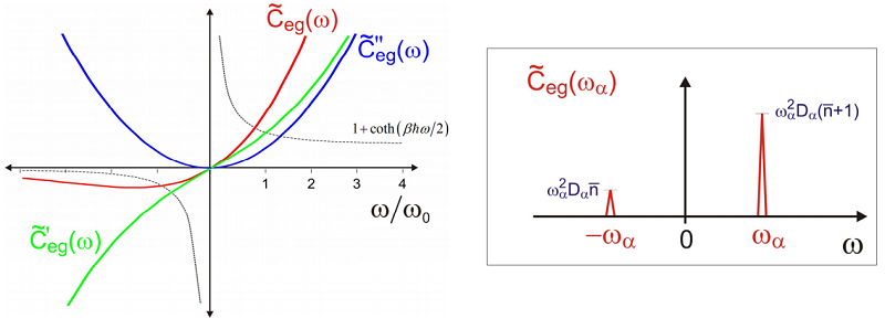
Here \(\tilde {C} _ {e s}^{\prime} ( \omega )\) and \(\tilde {C} _ {e g}^{\prime \prime} ( \omega )\) are the Fourier transforms of the real and imaginary components of \(C _ {e s} (t)\), respectively. \(\tilde {C} _ {e s}^{\prime} ( \omega )\) and \(\tilde {C} _ {e g}^{\prime \prime} ( \omega )\) are even and odd in frequency. Thus while \(\tilde {C} _ {e s} ( \omega )\) is entirely real valued, it is asymmetric about \(\omega = 0\).

With these definitions in hand, we can write the spectrum of the energy gap correlation function for coupling to a single harmonic mode spectrum (Equation \ref{13.71}):

\[\tilde {C} _ {e g} \left( \omega _ {\alpha} \right) = \omega _ {\alpha}^{2} D \left( \omega _ {\alpha} \right) \left[ \left( \overline {n} _ {\alpha} + 1 \right) \delta \left( \omega - \omega _ {\alpha} \right) + \overline {n} _ {\alpha} \delta \left( \omega + \omega _ {\alpha} \right) \right] \label{13.90}\]

This is a spectrum that characterizes how bath vibrational modes of a certain frequency and thermal occupation act to modify the observed energy of the system. The first and second terms in Equation \ref{13.90} describe upward and downward energy shifts of the system, respectively. Coupling to a vibration typically leads to an upshift of the energy gap transition energy since energy must be put into the system and bath. However, as with hot bands, when there is thermal energy available in the bath, it also allows for down-shifts in the energy gap. The net balance of upward and downward shifts averaged over the bath follows the detailed balance expression

\[\tilde {C} ( - \omega ) = e^{- \beta \hbar \omega} \tilde {C} ( \omega ) \label{13.91}\]

The balance of rates tends toward equal with increasing temperature. Fourier transforms of Equation \ref13.76} gives two other representations of the energy gap spectrum

\[\tilde {C} _ {e g}^{\prime} \left( \omega _ {\alpha} \right) = \omega _ {\alpha}^{2} D \left( \omega _ {\alpha} \right) \operatorname {coth} \left( \beta \hbar \omega _ {\alpha} / 2 \right) \left[ \delta \left( \omega - \omega _ {\alpha} \right) + \delta \left( \omega + \omega _ {\alpha} \right) \right] \label{13.92}\]

\[\tilde {C} _ {e g}^{\prime \prime} \left( \omega _ {\alpha} \right) = \omega _ {\alpha}^{2} D \left( \omega _ {\alpha} \right) \left[ \delta \left( \omega - \omega _ {\alpha} \right) + \delta \left( \omega + \omega _ {\alpha} \right) \right]. \label{13.93}\]

The representations in Equation \ref{13.90}, \ref{13.92}, and \ref{13.93} are not independent, but can be related to one another through

\[\tilde{C}_{e g}^{\prime}\left(\omega_{\alpha}\right)=\operatorname{coth}\left(\beta \hbar \omega_{\alpha} / 2\right) \tilde{C}_{e g}^{\prime \prime}\left(\omega_{\alpha}\right)\]

\[\tilde {C} _ {e g} \left( \omega _ {\alpha} \right) = \left( 1 + \operatorname {coth} \left( \beta \hbar \omega _ {\alpha} / 2 \right) \right) \tilde {C} _ {e g}^{\prime \prime} \left( \omega _ {\alpha} \right) \label{13.95}\]

That is, given either the real or imaginary part of the energy gap correlation spectrum, we can predict the other part. As we will see, this relationship is one manifestation of the fluctuationdissipation theorem that we address later. Due to its independence on temperature, the spectral density \(\tilde {C} _ {e g}^{\prime \prime} \left( \omega _ {\alpha} \right)\) is the commonly used representation.

Also from Equations.\ref{13.69} and \ref{13.87} we obtain the lineshape function as

\[\left.\begin{aligned} g (t) & = \int _ {- \infty}^{+ \infty} d \omega \frac {1} {2 \pi} \frac {\tilde {C} _ {e g} ( \omega )} {\omega^{2}} [ \exp ( - i \omega t ) + i \omega t - 1 ] \\ & = \int _ {0}^{\infty} d \omega \frac {\tilde {C} _ {e g}^{\prime \prime} ( \omega )} {\pi \omega^{2}} \left[ \operatorname {coth} \left( \frac {\beta \hbar \omega} {2} \right) ( 1 - \cos \omega t ) + i ( \sin \omega t - \omega t ) \right] \end{aligned} \right. \label{13.96}\]

The first expression relates g(t) to the complex energy gap correlation function, whereas the second separates the real and the imaginary parts and relates them to the imaginary part of the energy gap correlation function.

Coupling to a Harmonic Bath

More generally for condensed phase problems, the system coordinates that we observe in an experiment will interact with a continuum of nuclear motions that may reflect molecular vibrations, phonons, or intermolecular interactions. We describe this continuum as continuous distribution of harmonic oscillators of varying mode frequency and coupling strength. The Energy Gap Hamiltonian is readily generalized to the case of a continuous distribution of motions if we statistically characterize the density of states and the strength of interaction between the system and this bath. This method is also referred to as the Spin-Boson Model used for treating a two level spin-½ system interacting with a quantum harmonic bath.

Following our earlier discussion of the DHO model, the generalization of the EG Hamiltonian to the multimode case is

\[H _ {0} = \hbar \omega _ {e g} + H _ {e g} + H _ {B} \label{13.97}\]

\[H _ {B} = \sum _ {\alpha} \hbar \omega _ {\alpha} \left( p _ {\sim}^{2} + q _ {\alpha}^{2} \right) \label{13.98}\]

\[H _ {e g} = \sum _ {\alpha} 2 \hbar \omega _ {\alpha} d _ {\alpha} q _ {\alpha} + \lambda \label{13.99}\]

\[\lambda = \sum _ {\alpha} \hbar \omega _ {\alpha} d _ {\alpha}^{2} \label{13.100}\]

Note that the time-dependence to \(H_{eg}\) results from the interaction with the bath:

\[H _ {e g} (t) = e^{i H _ {B} t / \hbar} H _ {e g} e^{- i H _ {B} t / \hbar} \label{13.101}\]

Also, since the harmonic modes are normal to one another, the dephasing function and lineshape function are obtained from Equation \ref{13.102}

\[F(t)=\prod_{\alpha} F_{\alpha}(t) \quad g(t)=\sum_{\alpha} g_{\alpha}(t)\label{13.102}\]

For a continuum, we assume that the number of modes are so numerous as to be continuous, and that the sums in the equations above can be replaced by integrals over a continuous distribution of states characterized by a density of states W Z . Also the interaction with modes of a particular frequency are equal so that we can simply average over a frequency dependent coupling constant 2 D d Z Z . For instance, Equation \ref{13.102} becomes

\[g (t) = \int d \omega _ {\alpha} W \left( \omega _ {\alpha} \right) g \left( t , \omega _ {\alpha} \right) \label{13.103}\]

Coupling to a continuum leads to dephasing resulting from interaction to a continuum of modes of varying frequency. This will be characterized by damping of the energy gap frequency correlation function

\[C _ {e g} (t) = \int d \omega _ {\alpha} C _ {e g} \left( \omega _ {\alpha} , t \right) W \left( \omega _ {\alpha} \right) \label{13.104}\]

Here \(C _ {e g} \left( \omega _ {\alpha} , t \right) = \left\langle \delta \omega _ {e g} \left( \omega _ {\alpha} , t \right) \delta \omega _ {e g} \left( \omega _ {\alpha} , 0 \right) \right\rangle\) refers to the energy gap frequency correlation function for a single harmonic mode given in Equation \ref{13.71}. While Equation \ref{13.104} expresses the modulation of the energy gap in the time domain, we can alternatively express the continuous distribution of coupled bath modes in the frequency domain:

\[\tilde {C} _ {e g} ( \omega ) = \int d \omega _ {\alpha} W \left( \omega _ {\alpha} \right) \tilde {C} _ {e g} \left( \omega _ {\alpha} \right) \label{13.105}\]

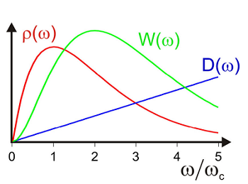
An integral of a single harmonic mode spectrum over a continuous density of states provides a coupling weighted density of states that reflects the action spectrum for the system-bath interaction. We evaluate this with the single harmonic mode spectrum, Equation \ref{13.90}. We see that the spectrum of the correlation function for positive frequencies is related to the product of the density of states and the frequency dependent coupling

\[\tilde{C}_{e g}(\omega)=\omega^{2} D(\omega) W(\omega)(\bar{n}+1) \quad(\omega>0) \label{13.106}\]

\[\tilde{C}_{e g}(\omega)=\omega^{2} D(\omega) W(\omega) \bar{n} \quad(\omega<0) \label{13.107}\]

This is an action spectrum that reflects the coupling weighted density of states of the bath that contributes to the spectrum.

In practice, the unusually symmetry of \(\tilde {C} _ {e g} ( \omega )\) and its growth as \(\omega^{2}\) make it difficult to work with. Therefore we choose to express the frequency domain representation of the coupling-weighted density of states in Equation \ref{13.106} as a spectral density, defined as

\[\left.\begin{aligned} \rho ( \omega ) & \equiv \frac {\tilde {C} _ {e g}^{\prime \prime} ( \omega )} {\pi \omega^{2}} \\ & = \frac {1} {\pi} \int d \omega _ {\alpha} W \left( \omega _ {\alpha} \right) D \left( \omega _ {\alpha} \right) \delta \left( \omega - \omega _ {\alpha} \right) \\ & = \frac {1} {\pi} W ( \omega ) D ( \omega ) \end{aligned} \right. \label{13.108}\]

This expression is real and defined only for positive frequencies. Note \(\tilde {C} _ {e g}^{\prime \prime} ( \omega )\) is an odd function in \(\infty\), and therefore \(\rho(\infty)\) is also.

Example of spectral density using an ohmic density of states, \(W ( \omega ) = \omega \exp \left[ - \omega / \omega _ {C} \right]\) and a linearly varying frequency dependent coupling.

The reorganization energy can be obtained from the first moment of the spectral density

\[\lambda = \hbar \int _ {0}^{\infty} d \omega \omega \rho ( \omega ) \label{13.109}\]

Furthermore, from Equation \ref{13.69} and \ref{13.105} we obtain the lineshape function in two forms

\[\left.\begin{aligned} g (t) & = \int _ {- \infty}^{+ \infty} d \omega \frac {1} {2 \pi} \frac {\tilde {C} _ {e g} ( \omega )} {\omega^{2}} [ \exp ( - i \omega t ) + i \omega t - 1 ] \\[4pt] & = - \frac {i \lambda t} {\hbar} + \int _ {0}^{\infty} d \omega \rho ( \omega ) \left[ \operatorname {coth} \left( \frac {\beta \hbar \omega} {2} \right) ( 1 - \cos \omega t ) + i \sin \omega t \right] \end{aligned} \right. \label{13.110}\]

In this expression the temperature dependence implies that in the high temperature limit, the real part of \(g(t)\) will dominate, as expected for a classical system. This is a perfectly general expression for the lineshape function in terms of an arbitrary spectral distribution describing the time scale and amplitude of energy gap fluctuations. Given a spectral density \(\rho(\infty)\), you can calculate various spectroscopic observables and other time-dependent processes in a fluctuating environment.

Now, let’s evaluate the behavior of the lineshape function and absorption lineshape for different forms of the spectral density. To keep things simple, we will consider the high temperature limit, \(k _ {B} T \ll \hbar \omega\). Here

\[\operatorname {coth} ( \beta \hbar \omega / 2 ) \rightarrow 2 / \beta \hbar \omega\]

and we can neglect the imaginary part of the frequency correlation function and lineshape function. These examples are motivated by the spectral densities observed for random or noisy processes. Depending on the frequency range and process of interest, noise tends to scale as \(U \approx Z^{-n}\), where \(n = 0\), \(1\) or \(2\). This behavior is often described in terms of a spectral density of the form

\[\rho ( \omega ) \propto \omega _ {c}^{1 - s} \omega^{s - 2} e^{- \omega / \omega _ {c}} \label{13.111}\]

where \(Z_c\) is a cut-off frequency, and the units are inverse frequency. These spectral densities have the desired property of being an odd function in \(Z\), and can be integrated to a finite value. The case \(s = 1\) is known as the Ohmic spectral density, whereas \(s > 1\) is super-ohmic and \(s < 1\) is sub-ohmic.

Step 1

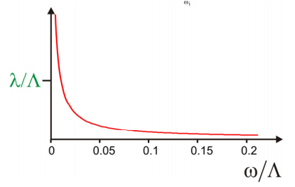
Let’s first consider the example when \(U\) drops as \(1/Z\) with frequency, which refers to the Ohmic spectral density with a high cut-off frequency. This is the spectral density that corresponds to an energy gap correlation function that decays infinitely fast: \(C_{e g}(t) \sim \delta(t)\). To choose a definition consistent with Equation \ref{13.109}, we set

\[\rho ( \omega ) = \lambda / \Lambda \hbar \omega \label{13.112}\]

where \(\Lambda\) is a finite high frequency integration limit that we enforce to keep \(U\) well behaved. \(\Lambda\) has units of frequency, it is equated with the inverse correlation time for the fast decay of \(C_{eg}(t)\).

Now we evaluate

\[\begin{aligned} g (t) & = \int _ {0}^{\infty} d \omega \frac {2 k _ {B} T} {\Lambda \hbar \omega} \rho ( \omega ) ( 1 - \cos \omega t ) - \frac {i \lambda t} {\hbar} \\ & = \int _ {0}^{\infty} d \omega \frac {2 \lambda k _ {B} T ( 1 - \cos \omega t )} {\omega^{2}} - \frac {i \lambda t} {\hbar} \\ & = \lambda \frac {\pi k _ {B} T} {\Lambda \hbar^{2}} t - \frac {i \lambda t} {\hbar} \end{aligned} \label{13.113}\]

Then we obtain the dephasing function

\[F (t) = e^{- \Gamma t} \label{13.114}\]

where we have defined the exponential damping constant as

\[\Gamma = \lambda \frac {\pi k T} {\Lambda \hbar^{2}} \label{13.115}\]

From this we obtain the absorption lineshape

\[\sigma _ {a b s} \propto \frac {\left| \mu _ {e g} \right|^{2}} {\left( \omega - \omega _ {e g} \right) + i \Gamma} \label{13.116}\]

Thus, a spectral density that scales as \(1 / \omega\) has a rapidly fluctuating bath and leads to a homogeneous Lorentzian lineshape with a half-width \(\Gamma\).

Step 2

Now take the case that we choose a Lorentzian spectral density centered at \(Z= 0\). To keep the proper odd function of \(Z\) and definition of \(O\) we write:

\[\rho ( \omega ) = \frac {\lambda} {\hbar \omega} \frac {\Lambda} {\omega^{2} + \Lambda^{2}} \label{13.117}\]

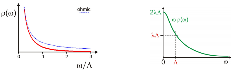
Note that for frequencies \(\omega \ll \Lambda\) this has the ohmic form of Equation \ref{13.112}. This is a spectral density that corresponds to an energy gap correlation function that drops exponentially as \(C_{e g}(t) \sim \exp (-\Lambda t)\). Here, in the high temperature (classical) limit \(k T>>\hbar \Lambda\), neglecting the imaginary part, we find

\[g (t) \approx \frac {\pi \lambda k T} {\hbar^{2} \Lambda^{2}} [ \exp ( - \Lambda t ) + \Lambda t - 1 ] \label{13.118}\]

This expression looks familiar. If we equate

\[\Delta^{2} = \lambda \frac {\pi k T} {\hbar^{2}} \label{13.119}\]

and

\[\tau _ {c} = \frac {1} {\Lambda} \label{13.120}\]

we obtain the same lineshape function as the classical Gaussian-stochastic model:

\[g (t) = \Delta^{2} \tau _ {c}^{2} \left[ \exp \left( - t / \tau _ {c} \right) + t / \tau _ {c} - 1 \right] \label{13.121}\]

So, the interaction of an electronic transition with a harmonic bath leads to line broadening that is equivalent to random fluctuations of the energy gap. As we noted earlier, for the homogeneous limit, we find \(\Gamma = \Delta^{2} \tau _ {c}\).

Readings

1. Mukamel, S., Principles of Nonlinear Optical Spectroscopy. Oxford University Press: New York, 1995; Ch. 7 and Ch. 8.