12.3: Different Types of Spectroscopy Emerge from the Dipole Operator

So the absorption spectrum in any frequency region is given by the Fourier transform over the dipole correlation function that describes the time-evolving change distributions in molecules, solids, and nanosystems. Let’s consider how this manifests itself in a few different spectroscopies, which have different contributions to the dipole operator. In general the dipole operator is a relatively simple representation of the charged particles of the system:

\[\vec{\mu} = \sum _ {i} q _ {i} \left( \vec{r} _ {i} - \vec{r} _ {0} \right) \label{11.29}\]

The complexity arises from the time-dependence of this operator, which evolves under the full Hamiltonian for the system:

\[\vec{\mu} (t) = e^{i H _ {0} t / \hbar} \vec{\mu} ( 0 ) e^{- i H _ {0} t / \hbar} \label{11.30}\]

where

\[\begin{align} H _ {0} = H _ {e l e c} + H _ {v i b} + H _ {r o t} + H _ {t r a n s} + H _ {s p i n} + \cdots + H _ {b a t h} + \cdots \\[4pt] + \sum _ {i , j \in [ e , v , r , t , s , b , E M \}} H _ {i - j} + \cdots \label{11.31} \end{align}\]

The full Hamiltonian accounts for the dynamics of all electronic, nuclear, and spin degrees of freedom. It is expressed in Equation \ref{11.31} in terms of separable contributions to all possible degrees of freedom and a bath Hamiltonian that contains all of the dark degrees of freedom not explicitly included in the dipole operator. We could also include an electromagnetic field. The last term describes pairwise couplings between different degrees of freedom, and emphasizes that interactions such as electron-nuclear interactions \(He_{e-v}\) and spin-orbit coupling \(He_{e-s}\). The wavefunction for the system can be expressed in terms of product states of the wavefunctions for the different degrees of freedom,

\[| \psi \rangle = | \psi _ {e l e c} \psi _ {v i b} \psi _ {r o t} \cdots \rangle \label{11.32}\]

When the \(H_{i-j}\) interaction terms are neglected, the correlation function can be separated into a product of correlation functions from various sources:

\[C _ {\mu \mu} (t) = C _ {e l e c} (t) C _ {v i b} (t) C _ {r o t} (t) \cdots \label{11.33}\]

which are each expressed in the form shown here for the vibrational states

\[C _ {\mu \mu} (t) = C _ {e l e c} (t) C _ {v i b} (t) C _ {r o t} (t) \cdots \label{11.34}\]

\(\Phi _ {n}\) is the wavefunction for the n^th vibrational eigenstate. The net correlation function will have oscillatory components at many frequencies and its Fourier transform will give the full absorption spectrum from the ultraviolet to the microwave regions of the spectrum. Generally speaking the highest frequency contributions (electronic or UV/Vis) will be modulated by contributions from lower frequency motions (… such as vibrations and rotations). However, we can separately analyze each of these contributions to the spectrum.

Atomic Transitions

\(H _ {0} = H _ {\text {atom}}\). For hydrogenic orbitals, \(| n \rangle \rightarrow | n \ell m _ {\ell} \rangle\).

Rotational Spectroscopy

From a classical perspective, the dipole moment can be written in terms of a permanent dipole moment with amplitude and direction

\[\vec{\mu} = \mu _ {0} \hat {u} \label{11.35}\]

\[\sigma ( \omega ) = \int _ {- \infty}^{+ \infty} d t e^{- i \omega t} \mu _ {0}^{2} \langle \hat {\varepsilon} \cdot \hat {u} ( 0 ) \hat {\varepsilon} \cdot \hat {u} (t) \rangle \label{11.36}\]

The lineshape is the Fourier transform of the rotational motion of the permanent dipole vector in the laboratory frame. \(\mu _ {0}\) is the magnitude of the permanent dipole moment averaged over the fast electronic and vibrational degrees of freedom. The frequency of the resonance would depend on the rate of rotation—the angular momentum and the moment of inertia. Collisions or other damping would lead to the broadening of the lines.

Quantum mechanically we expect a series of rotational resonances that mirror the thermal occupation and degeneracy of rotational states for the system. Taking the case of a rigid rotor with cylindrical symmetry as an example, the Hamiltonian is

\[H _ {m t} = \dfrac {\overline {L}^{2}} {2 I} \label{11.37}\]

and the wavefunctions are spherical harmonics, \(Y _ {J , M} ( \theta , \phi )\) which are described by

\[\overline {L}^{2} | Y _ {J , M} \rangle = \hbar^{2} J ( J + 1 ) | Y _ {J , M} \rangle \label{11.38A}\]

with \(J = 0,1,2 \ldots \label{11.38B}\) and

\[L _ {z} | Y _ {J , M} \rangle = M \hbar | Y _ {J , M} \rangle \label{11.38C}\]

with

\[M = - J , - J + 1 , \ldots , J \label{11.38D}\]

where \(J\) is the rotational quantum number and \(M\) (or \(M_J\)) refers to its projection onto an axis (z), and has a degeneracy of \(g_M(J)=2J+1\). The energy eigenvalues for Hrot are

\[E _ {J , M} = \tilde{B} J ( J + 1 ) \label{11.39}\]

where the rotational constant, here in units of joules, is

\[\tilde{B} = \frac {\hbar^{2}} {2 I} \label{11.40}\]

If we take a dipole operator in the form of Equation \ref{11.35}, then the far-infrared rotational spectrum will be described by the correlation function

\[ C _ {r o t} (t) = \sum _ {J , M} p _ {J , M} \left| \mu _ {0} \right|^{2} \left\langle Y _ {J , M} \left| e^{i H _ {m t} t h} ( \hat {u} \cdot \hat {\varepsilon} ) e^{- i H _ {m} t / h} ( \hat {u} \cdot \hat {\varepsilon} ) \right| Y _ {J , M} \right\rangle \label{11.41}\]

The evaluation of this correlation function involves an orientational average, which is evaluated as follows

\[ \left\langle Y _ {J , M} | f ( \theta , \phi ) | Y _ {J , M} \right\rangle = \frac {1} {4 \pi} \int _ {0}^{2 \pi} d \varphi \int _ {0}^{\pi} \sin \theta d \theta Y _ {J , M}^{*} f ( \theta , \phi ) Y _ {J , M} \label{11.42}\]

Recognizing that

\(\left( \hat {u} \cdot \hat {\varepsilon} _ {z} \right) = \cos \theta\), we can evaluate Equation \ref{11.41} using the reduction formula ,

\[\cos \theta | Y _ {J , M} \rangle = c _ {J +} | Y _ {J + 1 , M} \rangle + c _ {J -} | Y _ {J - 1 , M} \rangle \label{11.43}\]

with

\[c _ {J +} = \sqrt {\frac {( J + 1 )^{2} - M^{2}} {4 ( J + 1 )^{2} - 1}}\]

and

\[c _ {J -} = \sqrt {\frac {J^{2} + M^{2}} {4 J^{2} - 1}} \label{11.44}\]

and the orthogonality of spherical harmonics

\[\left\langle Y _ {J^{\prime} , M^{\prime}} | Y _ {J , M} \right\rangle = 4 \pi \delta _ {J , J} \delta _ {M^{\prime} , M} \label{11.45}\]

The factor \(p _ {J , M}\) in Equation \ref{11.41} is the probability of thermally occupying a particular \(J,\,M\) level. For this we recognize that

\[p _ {J , M} = g _ {M} ( J ) e^{- \beta E _ {J}} / Z _ {r o t}\]

so that Equation \ref{11.41} leads to the correlation function

\[\left\langle Y _ {J^{\prime} , M^{\prime}} | Y _ {J , M} \right\rangle = 4 \pi \delta _ {J , J} \delta _ {M^{\prime} , M} \label{11.46}\]

Fourier transforming Equation \ref{11.46} leads to the lineshape

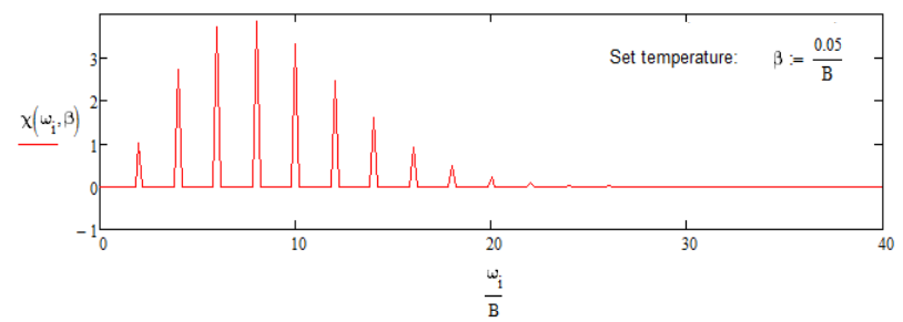
\[\sigma _ {r o t} ( \omega ) = \frac {\left| \mu _ {0} \right|^{2}} {Z _ {r o t}} \hbar \sum _ {J} ( 2 J + 1 ) e^{- \beta \overline {B} J ( J + 1 ) / \hbar} [ \delta ( \hbar \omega - 2 \overline {B} ( J + 1 ) ) + \delta ( \hbar \omega + 2 \overline {B} J ) ] \label{11.47}\]

The two terms reflect the fact that each thermally populated level with \(J > 0\) contributes both to absorptive and stimulated emission processes, and the observed intensity reflects the difference in populations.

IR Vibrational Spectroscopy

Vibrational spectroscopy can be described by taking the dipole moment to be weakly dependent on the displacement of vibrational coordinates

\[\overline {\mu} = \overline {\mu} _ {0} + \left. \frac {\partial \overline {\mu}} {\partial q} \right| _ {q = q _ {0}} q + \cdots \label{11.48}\]

Here the first expansion term is the permanent dipole moment and the second term is the transition dipole moment. If we are performing our ensemble average over vibrational states, the lineshape becomes the Fourier transform of a correlation function in the vibrational coordinate

\[\sigma ( \omega ) = \left| \frac {\partial \overline {\mu}} {\partial q} \right|^{2} \int _ {- \infty}^{+ \infty} d t \, e^{- i \omega t} \langle q ( 0 ) q (t) \rangle \label{11.49}\]

The vector nature of the transition dipole has been dropped here. So the time-dependent dynamics of the vibrational coordinate dictate the IR lineshape.

This approach holds for the classical and quantum mechanical cases. In the case of quantum mechanics, the change in charge distribution in the transition dipole moment is replaced with the equivalent transition dipole matrix element

\[| \partial \overline {\mu} / \partial q |^{2} \Rightarrow \left| \overline {\mu} _ {k \ell} \right|^{2}\]

If we take the vibrational Hamiltonian to be that of a harmonic oscillator,

\[H _ {v i b} = \frac {1} {2 m} p^{2} + \frac {1} {2} m \omega _ {0}^{2} q^{2} = \hbar \omega _ {0} \left( a^{\dagger} a + \frac {1} {2} \right)\]

then the time-dependence of the vibrational coordinate, expressed as raising and lowering operators is

\[q (t) = \sqrt {\frac {\hbar} {2 m \omega _ {0}}} \left( a^{\dagger} e^{i \omega _ {0} t} + a e^{- i \omega _ {0} t} \right)\]

The absorption lineshape is then obtained from Equation \ref{11.49}.

\[\sigma _ {v i b} ( \omega ) = \frac {1} {Z _ {v i b}} \sum _ {n} e^{- \beta n \hbar \omega _ {0}} \left[ \left| \overline {\mu} _ {( n + 1 ) n} \right|^{2} ( \overline {n} + 1 ) \delta \left( \omega - \omega _ {0} \right) + \left| \overline {\mu} _ {( n - 1 ) n} \right|^{2} \overline {n} \delta \left( \omega + \omega _ {0} \right) \right]\]

where \(\overline {n} = \left( e^{\beta \hbar \omega _ {0}} - 1 \right)^{- 1}\) is the thermal occupation number. For the low temperature limit applicable to most vibrations under room temperature conditions \(\overline {n} \rightarrow 0\) and

\[\sigma _ {v i b} ( \omega ) = \left| \overline {\mu} _ {10} \right|^{2} \delta \left( \omega - \omega _ {0} \right)\]

Raman Spectroscopy

Technically, we need second-order perturbation theory to describe Raman scattering, because transitions between two states are induced by the action of two light fields whose frequency difference equals the energy splitting between states. But much the same result is obtained is we replace the dipole operator with an induced dipole moment generated by the incident field: \(\overline {\mu} \Rightarrow \overline {\mu} _ {i n d}\). The incident field \(E_i\) polarizes the molecule,

\[\overline {\mu} _ {i n d} = \overline {\overline {\alpha}} \cdot \overline {E} _ {i} (t) \label{11.54}\]

(\(\overline {\alpha}\) is the polarizability tensor), and the scattered light field results from the interaction with this induced dipole

\[\begin{align} V (t) & = - \overline {\mu} _ {i n d} \cdot \overline {E} _ {s} (t) \\[4pt] & = \overline {E} _ {s} (t) \cdot \overline {\overline {\alpha}} \cdot \overline {E} _ {i} (t) \\[4pt] & = E _ {s} (t) E _ {i} (t) \left( \hat {\varepsilon} _ {s} \cdot \overline {\alpha} \cdot \hat {\varepsilon} _ {i} \right) \label{11.55} \end{align} \]

Here we have written the polarization components of the incident (\(i\)) and scattered (\(s\)) light projecting onto the polarizability tensor \( \overline{\overline {\alpha}}\). Equation \ref{11.55} leads to an expression for the Raman lineshape as

\[\begin{align} \sigma ( \omega ) &= \int _ {- \infty}^{+ \infty} d t e^{- i \omega t} \left\langle \hat {\varepsilon} _ {s} \cdot \overline {\alpha} ( 0 ) \cdot \hat {\varepsilon} _ {i} \hat {\varepsilon} _ {s} \cdot \overline {\overline {\alpha}} (t) \cdot \hat {\varepsilon} _ {i} \right\rangle \\[4pt] &= \int _ {- \infty}^{+ \infty} d t e^{- i \omega t} \langle \overline {\overline {\alpha}} ( 0 ) \overline {\overline {\alpha}} (t) \rangle \label{11.56} \end{align} \]

To evaluate this, the polarizability tensor can also be expanded in the nuclear coordinates

\[\overline {\overline {\alpha}} = \overline {\overline {\alpha} _ {0}} + \left. \frac {\partial \overline {\overline {\alpha}}} {\partial q} \right| _ {q = q _ {0}} q + \cdots \label{11.57}\]

where the leading term would lead to Raleigh scattering and rotational Raman spectra, and the second term would give vibrational Raman scattering. Also remember that the polarizability tensor is a second rank tensor that tells you how well a light field polarized along \(i\) can induce a dipole moment (light-field-induced charge displacement) in the s direction. For cylindrically symmetric systems which have a polarizability component \(\alpha _ {\|}\) along the principal axis of the molecule and a component \(\alpha _ {\perp}\) perpendicular to that axis, this usually takes the form

\[\overline {\overline {\alpha}} = \left( \begin{array} {c c} {\alpha _ {\|}} & {} \\ {} & {\alpha _ {\perp}} \\ {} & {} & {\alpha _ {\perp}} \end{array} \right) = \alpha \mathbf {I} + \frac {1} {3} \beta \left( \begin{array} {c c} {2} & {} \\ {} & {- 1} \\ {} & {} & {- 1} \end{array} \right) \label{11.58}\]

where \(\alpha\) is the isotropic component of polarizability tensor and \(\beta\) is the anisotropic component.