12.2: Time-Correlation Function Description of Absorption Lineshape

The interaction of light and matter as we have described from Fermi’s Golden Rule gives the rates of transitions between discrete eigenstates of the material Hamiltonian \(H_0\). The frequency dependence to the transition rate is proportional to an absorption spectrum. We also know that interaction with the light field prepares a superposition of the eigenstates of \(H_0\), and this leads to the periodic oscillation of amplitude between the states. Nonetheless, the transition rate expression really seems to hide any time-dependent description of motions in the system. An alternative approach to spectroscopy is to recognize that the features in a spectrum are just a frequency domain representation of the underlying molecular dynamics of molecules. For absorption, the spectrum encodes the time-dependent changes of the molecular dipole moment for the system, which in turn depends on the position of electrons and nuclei.

A time-correlation function for the dipole operator can be used to describe the dynamics of an equilibrium ensemble that dictate an absorption spectrum. We will make use of the transition rate expressions from first-order perturbation theory that we derived in the previous section to express the absorption of radiation by dipoles as a correlation function in the dipole operator. Let’s start with the rate of absorption and stimulated emission between an initial state \(| \ell \rangle\) and final state \(| k \rangle\) induced by a monochromatic field

\[w _ {k \ell} = \dfrac {\pi E _ {0}^{2}} {2 \hbar^{2}} | \langle k | \hat {\varepsilon} \cdot \overline {\mu} | \ell \rangle |^{2} \left[ \delta \left( \omega _ {k \ell} - \omega \right) + \delta \left( \omega _ {k \ell} + \omega \right) \right] \label{11.11}\]

For shorthand we have written

\[\left| \overline {\mu} _ {k \ell} \right|^{2} = | \langle k | \hat {\mathcal {E}} \cdot \overline {\mu} | \ell \rangle |^{2}.\]

We would like to use this to calculate the experimentally observable absorption coefficient (cross-section) which describes the transmission through the sample

\[T = \exp [ - \Delta N \alpha ( \omega ) L ] \label{11.12}\]

The absorption cross section describes the rate of energy absorption per unit time relative to the intensity of light incident on the sample

\[\alpha = \dfrac {- \dot {E} _ {r a d}} {I} \label{11.13}\]

The incident intensity is

\[I = \frac {c} {8 \pi} E _ {0}^{2} \label{11.14}\]

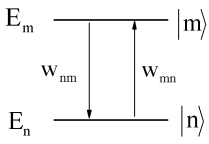
If we have two discrete states \(| m \rangle\) and \(| n \rangle\) with \(E _ {m} > E _ {n}\), the rate of energy absorption is proportional to the absorption rate and the transition energy

\[- \dot {E} _ {r a d} = w _ {n n} \cdot \hbar \omega _ {n m} \label{11.15}\]

For an ensemble this rate must be scaled by the probability of occupying the initial state.

More generally, we want to consider the rate of energy loss from the field as a result of the difference in rates of absorption and stimulated emission between states populated with a thermal distribution.

So, summing all possible initial and final states \(| \ell \rangle\) and \(| k \rangle\) over all possible upper and lower states \(| m \rangle\) and \(| n \rangle\) with

\[\left.\begin{aligned} - \dot {E} _ {\text {rad}} & = \sum _ {\ell , k \in [ m , n \}} p _ {\ell} w _ {k \ell} \hbar \omega _ {k \ell} \\ & = \dfrac {\pi E _ {0}^{2}} {2 \hbar} \sum _ {\ell , k \in [ m , n \}} \omega _ {k \ell} p _ {\ell} \left| \overline {\mu} _ {k \ell} \right|^{2} \left[ \delta \left( \omega _ {k \ell} - \omega \right) + \delta \left( \omega _ {k \ell} + \omega \right) \right] \end{aligned} \right. \label{11.16}\]

The cross section including the net change in energy as a result of absorption \(| n \rangle \rightarrow | m \rangle\) and stimulated emission \(| m \rangle \rightarrow | n \rangle\) is:

\[\alpha ( \omega ) = \dfrac {4 \pi^{2}} {\hbar c} \sum _ {n , m} \left[ \omega _ {m n} p _ {n} \left| \overline {\mu} _ {m n} \right|^{2} \delta \left( \omega _ {m n} - \omega \right) + \omega _ {n m} p _ {m} \left| \overline {\mu} _ {n m} \right|^{2} \delta \left( \omega _ {n m} + \omega \right) \right] \label{11.17}\]

To simplify Equation \ref{11.17}, we note:

1. Since \(\delta (x) = \delta ( - x )\), then \[\delta \left( \omega _ {n n} + \omega \right) = \delta \left( - \omega _ {m n} + \omega \right) = \delta \left( \omega _ {m n} - \omega \right).\]
2. The matrix elements squared in the two terms of Equation \ref{11.17} are the same: \[\left| \overline {\mu} _ {m n} \right|^{2} = \left| \overline {\mu} _ {n m} \right|^{2}.\]
3. and as a result of the delta function enforcing this equality: \[\omega _ {m n} = - \omega _ {n m} = \omega\]

So,

\[\alpha ( \omega ) = \dfrac {4 \pi^{2} \omega} {\hbar c} \sum _ {n , m} \left( p _ {n} - p _ {m} \right) \left| \overline {\mu} _ {m n} \right|^{2} \delta \left( \omega _ {m n} - \omega \right) \label{11.18}\]

Here we see that the absorption coefficient depends on the population difference between the two states. This is expected since absorption will lead to loss of intensity, whereas stimulated emission leads to gain. With equal populations in the upper and lower state, no change to the incident field would be expected. Since

\[p _ {n} - p _ {m} = p _ {n} \left( 1 - \exp \left[ - \beta \hbar \omega _ {m n} \right] \right) \label{11.19}\]

\[\alpha ( \omega ) = \dfrac {4 \pi^{2}} {\hbar c} \omega \left( 1 - e^{- \beta \hbar \omega} \right) \sum _ {n , m} p _ {n} \left| \overline {\mu} _ {m n} \right|^{2} \delta \left( \omega _ {m n} - \omega \right) \label{11.20}\]

Again the \(\omega _ {m n}\) factor has been replaced with \(\omega\). We can now separate \(\alpha\) into a product of factors that represent the field, and the matter, where the matter is described by \(\sigma ( \omega )\), the absorption lineshape.

\[\alpha ( \omega ) = \dfrac {4 \pi^{2}} {\hbar c} \omega \left( 1 - e^{- \beta \hbar \omega} \right) \sigma ( \omega ) \label{11.21}\]

\[\sigma ( \omega ) = \sum _ {n , m} p _ {n} \left| \overline {\mu} _ {m n} \right|^{2} \delta \left( \omega _ {m n} - \omega \right) \label{11.22}\]

To express the lineshape in terms of a correlation function we use one representation of the delta function through a Fourier transform of a complex exponential:

\[\delta \left( \omega _ {m n} - \omega \right) = \dfrac {1} {2 \pi} \int _ {- \infty}^{+ \infty} d t \,e^{i \left( \omega _ {m n} - \omega \right) t} \label{11.23}\]

to write

\[\sigma ( \omega ) = \dfrac {1} {2 \pi} \int _ {- \infty}^{+ \infty} d t \sum _ {n , m} p _ {n} \langle n | \overline {\mu} | m \rangle \langle m | \overline {\mu} | n \rangle e^{i \left( \omega _ {m n} - \omega \right) t} \label{11.24}\]

Now equating

\[U _ {0} | n \rangle = e^{- i H _ {0} t / \hbar} | n \rangle = e^{- i E _ {n} t / \hbar} | n \rangle\]

and recognizing that our expression contains the projection operator

\[\sigma ( \omega ) = \dfrac {1} {2 \pi} \int _ {- \infty}^{+ \infty} d t \sum _ {n , m} p _ {n} \langle n | \overline {\mu} | m \rangle \left\langle m \left| U _ {0}^{\dagger} \overline {\mu} U _ {0} \right| n \right\rangle e^{- i \omega t}\]

\[= \dfrac {1} {2 \pi} \int _ {- \infty}^{+ \infty} d t \sum _ {n , m} p _ {n} \left\langle n \left| \overline {\mu} _ {I} ( 0 ) \overline {\mu} _ {I} (t) \right| n \right\rangle e^{- i \omega t} \label{11.25}\]

But this last expression is just a dipole moment correlation function: the equilibrium thermal average over a pair of time-dependent dipole operators:

\[\sigma ( \omega ) = \dfrac {1} {2 \pi} \int _ {- \infty}^{+ \infty} d t e^{- i \omega t} \left\langle \overline {\mu} _ {I} ( 0 ) \overline {\mu} _ {I} (t) \right\rangle \label{11.26}\]

The absorption lineshape is given by the Fourier transform of the dipole correlation function. The correlation function describes the time-dependent behavior or spontaneous fluctuations in the dipole moment in absence of E field and contains information on states of system and broadening due to relaxation. Additional manipulations can be used to switch the order of operators by taking the complex conjugate of the exponential

\[\sigma ( \omega ) = \dfrac {1} {2 \pi} \int _ {- \infty}^{+ \infty} d t e^{i \omega t} \left\langle \overline {\mu} _ {I} (t) \overline {\mu} _ {I} ( 0 ) \right\rangle \label{11.27}\]

and we can add back the polarization of the light field to the matrix element

\[\sigma ( \omega ) = \dfrac {1} {2 \pi} \int _ {- \infty}^{+ \infty} d t e^{i \omega t} \left\langle \hat {\varepsilon} \cdot \overline {\mu} _ {I} (t) \hat {\varepsilon} \cdot \overline {\mu} _ {I} ( 0 ) \right\rangle \label{11.28}\]

to emphasize the orientational component to this correlation function. Here we have written operators emphasizing the interaction picture representation. As we move forward, we will drop this notation, and take it as understood that for the purposes of spectroscopy, the dipole operator is expressed in the interaction picture and evolves under the material Hamiltonian \(H_0\).

Readings

1. McHale, J. L., Molecular Spectroscopy. 1st ed.; Prentice Hall: Upper Saddle River, NJ, 1999.
2. McQuarrie, D. A., Statistical Mechanics. Harper & Row: New York, 1976; Ch. 21.
3. Nitzan, A., Chemical Dynamics in Condensed Phases. Oxford University Press: New York, 2006.
4. Schatz, G. C.; Ratner, M. A., Quantum Mechanics in Chemistry. Dover Publications: Mineola, NY, 2002; Section 6.2.