12.1: A Classical Description of Spectroscopy

The traditional quantum mechanical treatment of spectroscopy is a static representation of a very dynamic process. An oscillating light field acts to drive bound charges in matter, which under resonance conditions leads to efficient exchange of energy between the light and matter. This dynamical picture emerges from a time-domain description, which shares many similarities to a classical description. Since much of the physical intuition that is helpful in understanding spectroscopy naturally emerges from the classical view, we will describe it first.

The classical view begins with the observation that atoms and molecules are composed of charged particles, and these charges are the handle by which an electromagnetic field exerts a force on the atom or molecule. The force exerted on the molecules depends on the form of the potential binding the charges together, the magnitude of the charges, and the strength of the external field.

The simplest elements of a model that captures what happens in absorption spectroscopy require us to consider a charged particle in a bound potential interacting with an oscillating driving force. The matter can be expressed in terms of a particle with charge \(z\) in a harmonic potential (the leading term in any expansion of the potential in the coordinate \(Q\)):

\[V _ {r e s} (t) = \dfrac {1} {2} \kappa Q^{2} \label{11.1}\]

Here \(k\) is the restoring force constant. For the light field, we use the traditional expression

\[V _ {e x t} (t) = - \overline {\mu} \cdot \overline {E} (t) \label{11.2}\]

for an external electromagnetic field interacting with the dipole moment of the system, \(\overline {\mu} = z Q\). We describe the behavior of this system using Newton’s equation of motion F=ma, which we write as

\[m \dfrac {\partial^{2} Q} {\partial t^{2}} = F _ {r e s} + F _ {d a m p} + F _ {e x t} \label{11.3}\]

On the right hand side of Equation \ref{11.3} there are three forces: the harmonic restoring force, a damping force, and the driving force exerted by the light. Remembering that

\[F = - ( \partial V / \partial Q )\]

we can write Equation \ref{11.3} as

\[m \dfrac {\partial^{2} Q} {\partial t^{2}} = - \kappa Q - b \dfrac {\partial Q} {\partial t} + F _ {0} \cos ( \omega t ) \label{11.4}\]

Here, \(b\) describes the rate of damping. For the field, we have only considered the time-dependence

\[\overline {E} (t) = \overline {E} _ {0} \cos ( \omega t )\]

and the amplitude of the driving force

\[F _ {0} = \left( \dfrac {\partial \overline {\mu}} {\partial Q} \right) \cdot \overline {E} _ {0} \label{11.5}\]

Equation \ref{11.5} indicates that increasing the force on the oscillator is achieved by raising the magnitude of the field, increasing how much the charge is displaced, or improving the alignment between the electric field polarization and the transition dipole moment. We can rewrite Equation \ref{11.4} as the driven harmonic oscillator equation:

\[\dfrac {\partial^{2} Q} {\partial t^{2}} + 2 \gamma \dfrac {\partial Q} {\partial t} + \omega _ {0}^{2} Q = \dfrac {F _ {0}} {m} \cos ( \omega t ) \label{11.6}\]

Here the damping constant \(\gamma = b / 2 m\) and the harmonic resonance frequency \(\omega _ {0} = \sqrt {\kappa / m}\).

Let’s look at the solution to Equation \ref{11.6} for a couple of simple cases.

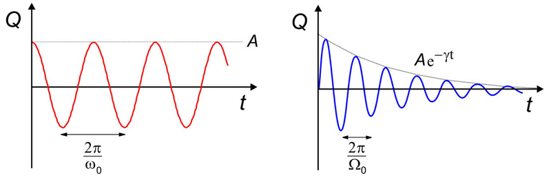
First, for the case (red curve) that there is no damping or driving force (\(\gamma = F _ {0} = 0\)), we have simple harmonic solutions in which oscillate at a frequency \(\omega _ {0}\):

\[Q (t) = A \sin \left( \omega _ {0} t \right) + B \cos \left( \omega _ {0} t \right)\]

Let’s just keep the \(sin\) term for now. Now if you add damping to the equation:

\[Q (t) = A e^{- \gamma t} \sin \Omega _ {0} t\]

The coordinate oscillates at a reduced frequency

\[\Omega _ {0} = \sqrt {\omega _ {0}^{2} - \gamma^{2}}\]

As we continue, let’s assume a case with weak damping for which \(\Omega _ {0} \approx \omega _ {0}\) (blue curve).

The solution to Equation \ref{11.6} takes the form

\[Q (t) = \dfrac {F _ {0} / m} {\sqrt {\left( \omega _ {0}^{2} - \omega^{2} \right)^{2} + 4 \gamma^{2} \omega^{2}}} \sin ( \omega t + \beta ) \label{11.7}\]

where the phase factor is

\[\tan \beta = \left( \omega _ {0}^{2} - \omega^{2} \right) / 2 \gamma \omega \label{11.8}\]

So this solution to the displacement of the particle says that the amplitude certainly depends on the magnitude of the driving force, but more importantly on the resonance condition. The frequency of the driving field should match the natural resonance frequency of the system, \(\omega _ {0} \approx \infty\) … like pushing someone on a swing. When you drive the system at the resonance frequency there will be an efficient transfer of power to the oscillator, but if you push with arbitrary frequency, nothing will happen. Indeed, that is what an absorption spectrum is: a measure of the power absorbed by the system from the field.

Notice that the coordinate oscillates at the driving frequency ω and not at the resonance frequency \(\omega_0\). Also, the particle oscillates as a sin, that is, 90° out-of-phase with the field when driven on resonance. This reflects the fact that the maximum force can be exerted on the particle when it is stationary at the turning points. The phase shift \(\beta\), depends varies with the detuning from resonance. Now we can make some simplifications to Equation \ref{11.7} and calculate the absorption spectrum. For weak damping \(\gamma < < \omega _ {0}\) and near resonance \(\omega _ {0} \approx \infty\), we can write

\[\left( \omega _ {0}^{2} - \omega^{2} \right)^{2} = \left( \omega _ {0} - \omega \right)^{2} \left( \omega _ {0} + \omega \right)^{2} \approx 4 \omega _ {0}^{2} \left( \omega _ {0} - \omega \right)^{2} \label{11.9}\]

The absorption spectrum is a measure of the power transferred to the oscillator, so we can calculate it by finding the power absorbed from the force on the oscillator times the velocity, averaged over a cycle of the field.

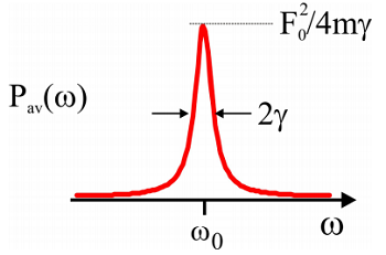
\[ \begin{align} P _ {a v g} &= \left\langle F (t) \cdot \dfrac {\partial Q} {\partial t} \right\rangle _ {a v g} \\[4pt] &= \dfrac {\gamma F _ {0}^{2}} {2 m} \dfrac {1} {\left( \omega - \omega _ {0} \right)^{2} + \gamma^{2}} \label{11.10} \end{align}\]

This is the Lorentzian lineshape, which is peaked at the resonance frequency and has a line width of \(2\gamma\) (full width half-maximum, FWHM). The area under the lineshape is \(\pi F _ {0}^{2} / 4 m\).