11.1: Classical Linear Response Theory

We will use linear response theory as a way of describing a real experimental observable. Specifically this will tell us how an equilibrium system changes in response to an applied potential. The quantity that will describe this is a response function, a real observable quantity. We will go on to show how it is related to correlation functions. Embedded in this discussion is a particularly important observation. We will now deal with a nonequilibrium system, but we will show that when the changes are small away from equilibrium, the equilibrium fluctuations dictate the nonequilibrium response! Thus knowledge of equilibrium dynamics is useful in predicting the outcome of nonequilibrium processes.

So, the question is “How does the system respond if you drive it away from equilibrium?” We will examine the case where an equilibrium system, described by a Hamiltonian \(H_0\) interacts weakly with an external agent, \(V(t)\). The system is moved away from equilibrium by the external agent, and the system absorbs energy from the external agent. How do we describe the time-dependent properties of the system? We first take the external agent to interact with the system through an internal variable \(A\). So the Hamiltonian for this problem is given by

\[H = H _ {0} - f (t) A \label{10.1}\]

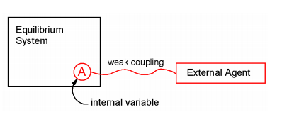
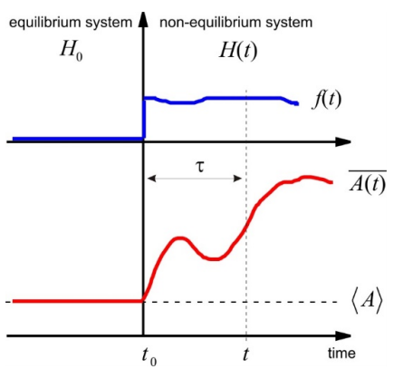
Here \(f(t)\) is the time-dependent action of the external agent, and the deviation from equilibrium is linear in the internal variable. We describe the behavior of an ensemble initially at thermal equilibrium by assuming that each member of the ensemble is subject to the same interaction with the external agent, and then ensemble averaging. Initially, the system is described by \(H_0\). It is at equilibrium and the internal variable is characterized by an equilibrium ensemble average \(\langle A \rangle\). The external agent is then applied at time t0, and the system is moved away from equilibrium, and is characterized through a nonequilibrium ensemble average, \(\overline {A}\). \(\langle A \rangle \neq \overline {A (t)}\) as a result of the interaction.

For a weak interaction with the external agent, we can describe \(\overline {A (t)}\) by performing an expansion in powers of \(f(t)\)

\[\begin{align} \overline {A (t)} &= \left( \text {terms} f^{( 0 )} \right) + \left( \text {terms} f^{( 1 )} \right) + \ldots \label{10.2} \\[4pt] &= \langle A \rangle + \int d t _ {0} R \left( t , t _ {0} \right) f \left( t _ {0} \right) + \ldots \label{10.3} \end{align}\]

In this expression the agent is applied at 0 t , and we observe the system att. The leading term in this expansion is independent of f, and is therefore equal to A . The next term in Equation \ref{10.3} describes the deviation from the equilibrium behavior in terms of a linear dependence on the external agent. \(R \left( t , t _ {0} \right)\) is the linear response function, the quantity that contains the microscopic information on the system and how it responds to the applied agent. The integration in the last term of Equation \ref{10.3} indicates that the nonequilibrium behavior depends on the full history of the application of the agent \(f \left( t _ {0} \right)\) and the response of the system to it. We are seeking a quantum mechanical description of \(R\).

Properties of the Response Function

1. Causal: Causality refers to the common sense observation that the system cannot respond before the force has been applied. Therefore \(R \left( t , t _ {0} \right) = 0\) for \(t < t\), and the time-dependent change in \(A\) is

\[\overline {\delta A (t)} = \overline {A (t)} - \langle A \rangle = \int _ {- \infty}^{t} d t _ {0} R \left( t , t _ {0} \right) f \left( t _ {0} \right) \label{10.4}\]

The lower integration limit is set to \(- \infty\) to reflect that the system is initially at equilibrium, and the upper limit is the time of observation. We can also make the statement of causality explicit by writing the linear response function with a step response: \(\Theta \left( t - t _ {0} \right) R \left( t , t _ {0} \right)\), where

\[\Theta \left( t - t _ {0} \right) \equiv \left\{\begin{array} {l l} {0} & {\left( t < t _ {0} \right)} \\ {1} & {\left( t \geq t _ {0} \right)} \end{array} \right. \label{10.5}\]

2. Stationary: Similar to our discussion of correlation functions, the time-dependence of the system only depends on the time interval between application of the potential and observation. Therefore we write

\[R \left( t , t _ {0} \right) = R \left( t - t _ {0} \right)\]

and

\[\delta \overline {A (t)} = \int _ {- \infty}^{t} d t _ {0} R \left( t - t _ {0} \right) f \left( t _ {0} \right) \label{10.6}\]

This expression says that the observed response of the system to the agent is a convolution of the material response with the time-development of the applied force. Rather than the absolute time points, we can define a time-interval \(\tau = t - t _ {0}\), so that we can write

\[\delta \overline {A (t)} = \int _ {0}^{\infty} d \tau R ( \tau ) f ( t - \tau ) \label{10.7}\]

3. Impulse response: Note that for a delta function perturbation:

\[f (t) = \lambda \delta \left( t - t _ {0} \right) \label{10.8}\]

We obtain

\[\overline {\delta A (t)} = \lambda R \left( t - t _ {0} \right) \label{10.9}\]

Thus, \(R\) describes how the system behaves when an abrupt perturbation is applied and is often referred to as the impulse response function. An impulse response kicks the system away from the equilibrium established under H0, and therefore the shape of a response function will always rise from zero and ultimately return to zero. In other words, it will be a function that can be expanded in sines. Thus the response to an arbitrary f(t) can be described through a Fourier analysis, suggesting that a spectral representation of the response function would be useful.

The Susceptibility

The observed temporal behavior of the nonequilibrium system can also be cast in the frequency domain as a spectral response function, or susceptibility. We start with Equation \ref{10.7} and Fourier transform both sides:

\[\left.\begin{aligned} \overline {\delta A ( \omega )} & \equiv \int _ {- \infty}^{+ \infty} d t \delta \overline {A (t)} e^{i \omega t} \\ & = \int _ {- \infty}^{+ \infty} d t \left[ \int _ {0}^{\infty} d \tau R ( \tau ) f ( t - \tau ) \right] e^{i \omega t} \end{aligned} \right. \label{10.10}\]

Now we insert \(e^{- i \omega \tau} e^{+ i \omega \tau} = 1\) and collect terms to give

\[ \begin{align} \delta \overline {A ( \omega )} &= \int _ {- \infty}^{+ \infty} d t \int _ {0}^{\infty} d \tau R ( \tau ) f ( t - \tau ) e^{i \omega ( t - \tau )} e^{i \omega \tau} \label{10.11} \\[4pt] &= \int _ {- \infty}^{+ \infty} d t^{\prime} e^{i \omega r^{\prime}} f \left( t^{\prime} \right) \int _ {0}^{\infty} d \tau R ( \tau ) e^{i \omega \tau} \label{10.12} \end{align}\]

or

\[\delta \overline {A ( \omega )} = \tilde {f} ( \omega ) \chi ( \omega ) \label{10.13}\]

In Equation \ref{10.12} we switched variables, setting \(t^{\prime} = t - \tau\). The first term \(\tilde {f} ( \omega )\) is a complex frequency domain representation of the driving force, obtained from the Fourier transform of \(f \left( t^{\prime} \right)\). The second term \(\chi ( \omega )\) is the susceptibility which is defined as the Fourier–Laplace transform (i.e., single-sided Fourier transform) of the impulse response function. It is a frequency domain representation of the linear response function. Switching between time and frequency domains shows that a convolution of the force and response in time leads to the product of the force and response in frequency. This is a manifestation of the convolution theorem:

\[A (t) \otimes B (t) \equiv \int _ {- \infty}^{\infty} d \tau A ( t - \tau ) B ( \tau ) = \int _ {- \infty}^{\infty} d \tau A ( \tau ) B ( t - \tau ) = \mathcal {H}^{- 1} [ \tilde {A} ( \omega ) \tilde {B} ( \omega ) ] \label{10.14}\]

Here \(\otimes\) refers to convolution, \(\tilde {A} ( \omega ) = \mathcal {F} [ A (t) ]] \), \(\mathcal {F}\) is a Fourier transform, and \(\mathcal {F}^{- 1} [ \cdots ]\) is an inverse Fourier transform.

Note that \(R(\tau)\) is a real function, since the response of a system is an observable. The susceptibility \(\chi ( \omega )\) is complex:

\[\chi ( \omega ) = \chi^{\prime} ( \omega ) + i \chi^{\prime \prime} ( \omega ) \label{10.15}\]

Since

\[\chi ( \omega ) = \int _ {0}^{\infty} d \tau R ( \tau ) e^{i \omega \tau} \label{10.16}\]

However, the real and imaginary contributions are not independent. We have

\[\chi^{\prime} = \int _ {0}^{\infty} d \tau R ( \tau ) \cos \omega \tau \label{10.17}\]

and

\[\chi^{\prime \prime} = \int _ {0}^{\infty} d \tau R ( \tau ) \sin \omega \tau \label{10.18}\]

\(\chi^{\prime}\) and \(\chi^{\prime \prime}\) are even and odd functions of frequency:

\[\chi^{\prime} ( \omega ) = \chi^{\prime} ( - \omega ) \label{10.19}\]

\[\chi^{\prime \prime} ( \omega ) = - \chi^{\prime \prime} ( - \omega ) \label{10.20}\]

so that \[\chi ( - \omega ) = \chi^{*} ( \omega ) \label{10.21}\]

Notice also that Equation \ref{10.21} allows us to write

\[\chi^{\prime} ( \omega ) = \frac {1} {2} [ \chi ( \omega ) + \chi ( - \omega ) ] \label{10.22}\]

\[\chi^{\prime \prime} ( \omega ) = \frac {1} {2 i} [ \chi ( \omega ) - \chi ( - \omega ) ] \label{10.23}\]

Kramers–Krönig relations

Since they are cosine and sine transforms of the same function, \(\chi^{\prime} ( \omega )\) is not independent of \(\chi^{\prime \prime} ( \omega )\). The two are related by the Kramers–Krönig relationships:

\[\begin{align} \chi^{\prime} ( \omega ) &= \frac {1} {\pi} P \int _ {- \infty}^{+ \infty} \frac {\chi^{\prime \prime} \left( \omega^{\prime} \right)} {\omega^{\prime} - \omega} d \omega^{\prime} \label{10.24} \\[4pt] \chi^{\prime \prime} ( \omega ) &= - \frac {1} {\pi} P \int _ {- \infty}^{+ \infty} \frac {\chi^{\prime} \left( \omega^{\prime} \right)} {\omega^{\prime} - \omega} d \omega^{\prime} \label{10.25} \end{align}\]

These are obtained by substituting the inverse sine transform of Equation \ref{10.18} into Equation \ref{10.17}

\[\begin{align} \chi^{\prime} ( \omega ) &= \frac {1} {\pi} \int _ {0}^{\infty} d t \cos \omega t \int _ {- \infty}^{+ \infty} \chi^{\prime \prime} \left( \omega^{\prime} \right) \sin \omega^{\prime} t d \omega^{\prime} \\[4pt] &= \frac {1} {\pi} \lim _ {L \rightarrow \infty} \int _ {- \infty}^{+ \infty} d \omega^{\prime} \chi^{\prime \prime} \left( \omega^{\prime} \right) \int _ {0}^{L} \cos \omega t \sin \omega^{\prime} t \,d t \end{align}\]

Using \(\cos a x \sin b x=\frac{1}{2} \sin (a+b) x+\frac{1}{2} \sin (b-a) x\) this can be written as

\[\chi^{\prime} ( \omega ) = \frac {1} {\pi} \lim _ {L \rightarrow \infty} \mathrm {P} \int _ {- \infty}^{+ \infty} d \omega^{\prime} \chi^{\prime \prime} ( \omega ) \frac {1} {2} \left[ \frac {- \cos \left( \omega^{\prime} + \omega \right) L + 1} {\omega^{\prime} + \omega} - \frac {\cos \left( \omega^{\prime} - \omega \right) L + 1} {\omega^{\prime} - \omega} \right] \label{10.27}\]

If we choose to evaluate the limit \(L \rightarrow \infty\), the cosine terms are hard to deal with, but we expect they will vanish since they oscillate rapidly. This is equivalent to averaging over a monochromatic field. Alternatively, we can average over a single cycle: \(L=2 \pi /\left(\omega^{\prime}-\omega\right)\) to obtain eq. (10.24). The other relation can be derived in a similar way. Note that the Kramers– Krönig relationships are a consequence of causality, which dictate the lower limit of \(T_{tinitial}=0\) on the first integral evaluated above.

Example \(\PageIndex{1}\): Driven Harmonic Oscillator

One can classically model the absorption of light through a resonant interaction of the electromagnetic field with an oscillating dipole, using Newton’s equations for a forced damped harmonic oscillator:

\[\ddot {x} - \gamma \dot {x} + \omega _ {0}^{2} x = F (t) / m \label{10.28}\]

Here the \(x\) is the coordinate being driven, \(\gamma\) is the damping constant, and \(\omega_{0}=\sqrt{k / m}\) is the natural frequency of the oscillator. We originally solved this problem is to take the driving force to have the form of a monochromatic oscillating source

\[F (t) = F _ {0} \cos \omega t \label{10.29}\]

Then, Equation \ref{10.28} has the solution

\[x (t) = \frac {F _ {0}} {m} \left( \left( \omega^{2} - \omega _ {0}^{2} \right)^{2} + \gamma^{2} \omega^{2} \right)^{- 1 / 2} \sin ( \omega t + \delta ) \label{10.30}\]

with

\[\tan \delta = \omega _ {0}^{2} - \omega^{2} / \gamma \omega \label{10.31}\]

This shows that the driven oscillator has an oscillation period that is dictated by the driving frequency \(\omega\), and whose amplitude and phase shift relative to the driving field is dictated by its detuning from resonance. If we cycle-average to obtain the average absorbed power from the field, the absorption spectrum is

\[\begin{align*} P _ {a v g} ( \omega ) &= \langle F (t) \cdot \dot {x} (t) \rangle \label{10.32} \\[4pt] &= = \frac {\gamma \omega^{2} F _ {0}^{2}} {2 m} \left[ \left( \omega _ {0}^{2} - \omega^{2} \right)^{2} + \gamma^{2} \omega^{2} \right]^{- 1 / 2} \end{align*}\]

To determine the response function for the damped harmonic oscillator, we seek a solution to Equation \ref{10.28} using an impulsive driving force

\[F (t) = F _ {0} \delta \left( t - t _ {0} \right) \nonumber\]

The linear response of this oscillator to an arbitrary force is

\[x (t) = \int _ {0}^{\infty} d \tau R ( \tau ) F ( t - \tau ) \label{10.33}\]

so that time-dependence with an impulsive driving force is directly proportional to the response function, \(x(t)=F_{0} R(t)\). For this case, we obtain

\[R ( \tau ) = \frac {1} {m \Omega} \exp \left( - \frac {\gamma} {2} \tau \right) \sin \Omega \tau \label{10.34}\]

The reduced frequency is defined as

\[\Omega = \sqrt {\omega _ {0}^{2} - \gamma^{2} / 4} \label{10.35}\]

From this, we evaluate eq. (10.16) and obtain the susceptibility

\[\chi ( \omega ) = \frac {1} {m \left( \omega _ {0}^{2} - \omega^{2} - i \gamma \omega \right)} \label{0.36}\]

As we will see shortly, the absorption of light by the oscillator is proportional to the imaginary part of the susceptibility

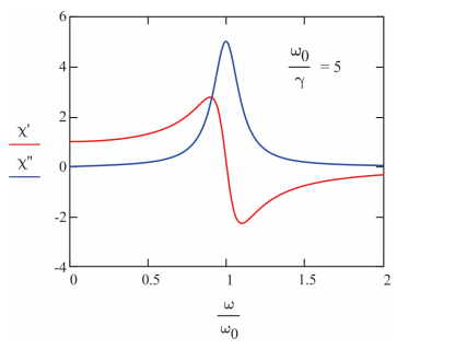
\[\chi^{\prime \prime} ( \omega ) = \frac {\gamma \omega} {m \left[ \left( \omega _ {0}^{2} - \omega^{2} \right)^{2} + \gamma^{2} \omega^{2} \right]} \label{10.37}\]

The real part is

\[\chi^{\prime} ( \omega ) = \frac {\omega _ {0}^{2} - \omega^{2}} {m \left[ \left( \omega _ {0}^{2} - \omega^{2} \right)^{2} + \gamma^{2} \omega^{2} \right]} \label{10.38}\]

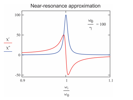
For the case of weak damping \(\gamma < < \omega _ {0}\) commonly encountered in molecular spectroscopy, Equation \ref{10.36} is written as a Lorentzian lineshape by using the near-resonance approximation

\[\omega^{2} - \omega _ {0}^{2} = \left( \omega + \omega _ {0} \right) \left( \omega - \omega _ {0} \right) \approx 2 \omega \left( \omega - \omega _ {0} \right) \label{10.39}\]

\[\chi ( \omega ) \approx \frac {1} {2 m \omega _ {0}} \frac {1} {\omega - \omega _ {0} + i \gamma / 2} \label{10.40}\]

Then the imaginary part of the susceptibility shows asymmetric lineshape with a line width of \(\gamma\) full width at half maximum.

\[\chi^{\prime \prime} ( \omega ) \approx \frac {1} {2 m \omega _ {0}} \frac {\gamma} {\left( \omega - \omega _ {0} \right)^{2} + \gamma^{2} / 4} \label{10.41}\]

\[\chi^{\prime} ( \omega ) \approx \frac {1} {m \omega _ {0}} \frac {\left( \omega - \omega _ {0} \right)} {\left( \omega - \omega _ {0} \right)^{2} + \gamma^{2} / 4} \label{10.42}\]

Nonlinear Response Functions

If the system does not respond in a manner linearly proportional to the applied potential but still perturbative, we can include nonlinear terms, i.e. higher expansion orders of \(\overline {A (t)}\) in Equation \ref{10.3}.

Let’s look at second order:

\[\delta \overline {A (t)}^{( 2 )} = \int d t _ {1} \int d t _ {2} R^{( 2 )} \left( t ; t _ {1} , t _ {2} \right) f _ {1} \left( t _ {1} \right) f _ {2} \left( t _ {2} \right) \label{10.43}\]

Again we are integrating over the entire history of the application of two forces \(f_1\) and \(f_2\), including any quadratic dependence on \(f\). In this case, we will enforce causality through a time ordering that requires

1. that all forces must be applied before a response is observed and
2. that the application of \(f_2\) must follow \(f_1\). That is \(t \geq t _ {2} \geq t _ {1}\) or

\[R^{( 2 )} \left( t ; t _ {1} , t _ {2} \right) \Rightarrow R^{( 2 )} \cdot \Theta \left( t - t _ {2} \right) \cdot \Theta \left( t _ {2} - t _ {1} \right) \label{10.44}\]

which leads to

\[\delta \overline {A (t)}^{( 2 )} = \int _ {- \infty}^{t} d t _ {2} \int _ {- \infty}^{t _ {2}} d t _ {1} R^{( 2 )} \left( t ; t _ {1} , t _ {2} \right) f _ {1} \left( t _ {1} \right) f _ {2} \left( t _ {2} \right) \label{10.45}\]

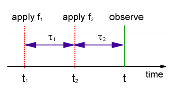
Now we will call the system stationary so that we are only concerned with the time intervals between consecutive interaction times. If we define the intervals between adjacent interactions

\[ \left. \begin{array} {l} {\tau _ {1} = t _ {2} - t _ {1}} \\ {\tau _ {2} = t - t _ {2}} \end{array} \right. \label{10.46} \]

Then we have

\[\delta \overline {A (t)}^{( 2 )} = \int _ {0}^{\infty} d \tau _ {1} \int _ {0}^{\infty} d \tau _ {2} R^{( 2 )} \left( \tau _ {1} , \tau _ {2} \right) f _ {1} \left( t - \tau _ {1} - \tau _ {2} \right) f _ {2} \left( t - \tau _ {2} \right) \label{10.47}\]

Readings

1. Berne, B. J., Time-Dependent Propeties of Condensed Media. In Physical Chemistry: An Advanced Treatise, Vol. VIIIB, Henderson, D., Ed. Academic Press: New York, 1971.
2. Berne, B. J.; Pecora, R., Dynamic Light Scattering. R. E. Krieger Publishing Co.: Malabar, FL, 1990.
3. Chandler, D., Introduction to Modern Statistical Mechanics. Oxford University Press: New York, 1987.
4. Mazenko, G., Nonequilibrium Statistical Mechanics. Wiley-VCH: Weinheim, 2006.
5. Slichter, C. P., Principles of Magnetic Resonance, with Examples from Solid State Physics. Harper & Row: New York, 1963.
6. Wang, C. H., Spectroscopy of Condensed Media: Dynamics of Molecular Interactions. Academic Press: Orlando, 1985.
7. Zwanzig, R., Nonequilibrium Statistical Mechanics. Oxford University Press: New York, 2001.

Contributors and Attributions

• Template:ContribTokmakoff