10.1: Definitions, Properties, and Examples of Correlation Functions

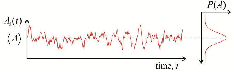
Returning to the microscopic fluctuations of a molecular variable \(A\), there seems to be little information in observing the trajectory for a variable characterizing the time-dependent behavior of an individual molecule. However, this dynamics is not entirely random, since they are a consequence of time-dependent interactions with the environment. We can provide a statistical description of the characteristic time scales and amplitudes to these changes by comparing the value of \(A\) at time \(t\) with the value of \(A\) at time \(t’\) later.

Figure \(\PageIndex{1}\): Fluctuations of \(A\) in time around an average \(\langle A \rangle \).

We define a time-correlation function (TCF) as a time-dependent quantity, \(A(t)\), multiplied by that quantity at some later time, \(A(t')\), and averaged over an equilibrium ensemble:

\[C _ {A A} \left( t , t^{\prime} \right) \equiv \left\langle A (t) A \left( t^{\prime} \right) \right\rangle _ {e q}\label{9.1}\]

The classical form of the correlation function is evaluated as

\[C _ {A A} \left( t , t^{\prime} \right) = \int d \mathbf {p} \int d \mathbf {q} A ( \mathbf {p} , \mathbf {q} ; t ) A \left( \mathbf {p} , \mathbf {q} ; t^{\prime} \right) \rho _ {e q} ( \mathbf {p} , \mathbf {q} ) \label{9.2}\]

whereas the quantum correlation function can be evaluated as

\[\begin{align} C _ {A A} \left( t , t^{\prime} \right) &= \operatorname {Tr} \left[ \rho _ {e q} A (t) A \left( t^{\prime} \right) \right] \\[4pt] &= \sum _ {n} p _ {n} \left\langle n \left| A (t) A \left( t^{\prime} \right) \right| n \right\rangle \label{9.3} \end{align}\]

where

\[p _ {n} = e^{- \beta E _ {n}} / Z.\]

These are auto-correlation functions, which correlates the same variable at two points in time, but one can also define a cross-correlation function that describes the correlation of two different variables in time

\[C _ {A B} \left( t , t^{\prime} \right) \equiv \left\langle A (t) B \left( t^{\prime} \right) \right\rangle \label{9.4}\]

So, what does a time-correlation function tell us? Qualitatively, a TCF describes how long a given property of a system persists until it is averaged out by microscopic motions and interactions with its surroundings. It describes how and when a statistical relationship has vanished. We can use correlation functions to describe various time-dependent chemical processes. For instance, we will use \(\langle \mu (t) \mu ( 0 ) \rangle\) - the dynamics of the molecular dipole moment - to describe absorption spectroscopy. We will also use them for relaxation processes induced by the interaction of a system and bath:

\[\left\langle H _ {S B} (t) H _ {S B} ( 0 ) \right\rangle.\]

Classically, you can use TCFs to characterize transport processes. For instance a diffusion coefficient is related to the velocity correlation function:

\[D = \frac {1} {3} \int _ {0}^{\infty} d t \langle v (t) v ( 0 ) \rangle.\]

Properties of Correlation Functions

A typical correlation function for random fluctuations at thermal equilibrium in the variable \(A\) might look like

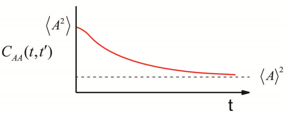
It is described by a number of properties:

1. When evaluated at \(t = t’\), we obtain the maximum amplitude, the mean square value of \(A\), which is positive for an autocorrelation function and independent of time. \[C _ {A A} ( t , t ) = \langle A (t) A (t) \rangle = \left\langle A^{2} \right\rangle \geq 0 \label{9.5}\]
2. For long time separations, as thermal fluctuations act to randomize the system, the values of A become uncorrelated \[\lim _ {t \rightarrow \infty} C _ {A A} \left( t , t^{\prime} \right) = \langle A (t) \rangle \left\langle A \left( t^{\prime} \right) \right\rangle = \langle A \rangle^{2} \label{9.6}\]
3. Since it is an equilibrium quantity, correlation functions are stationary. That means they do not depend on the absolute point of observation (\(t\) and \(t’\)), but rather the time interval between observations. A stationary random process means that the reference point can be shifted by an arbitrary value \(T\) \[C _ {A A} \left( t , t^{\prime} \right) = C _ {A A} \left( t + T , t^{\prime} + T \right) \label{9.7}\] So, choosing \(T = - t^{\prime}\) and defining the time interval \(\tau \equiv t - t^{\prime}\), we see that only \(\tau\) matters \[C _ {A A} \left( t , t^{\prime} \right) = C _ {A A} \left( t - t^{\prime} , 0 \right) = C _ {A A} ( \tau ) \label{9.8}\] Implicit in this statement is an understanding that we take the time-average value of \(A\) to be equal to the equilibrium ensemble average value of \(A\), i.e., the system is ergodic. So, the correlation of fluctuations can be expressed as either a time-average over a trajectory of one molecule \[\overline {A (t) A ( 0 )} = \lim _ {T \rightarrow \infty} \frac {1} {T} \int _ {0}^{T} d \tau A _ {i} ( t + \tau ) A _ {i} ( \tau ) \label{9.9}\] or an equilibrium ensemble average \[\langle A (t) A ( 0 ) \rangle = \sum _ {n} \frac {e^{- \beta E _ {n}}} {Z} \langle n | A (t) A ( 0 ) | n \rangle \label{9.10}\]
4. Classical correlation functions are real and even in time: \[\begin{align} \left\langle A (t) A \left( t^{\prime} \right) \right\rangle &= \left\langle A \left( t^{\prime} \right) A (t) \right\rangle \\[4pt] C _ {A A} ( \tau ) &= C _ {A A} ( - \tau ) \label{9.11} \end{align}\]
5. When we observe fluctuations about an average (Figure \(\PageIndex{1}\)), we often redefine the correlation function in terms of the deviation from average \[\delta A \equiv A - \langle A \rangle \label{9.12}\] and \[C _ {\delta A \delta A} (t) = \langle \delta A (t) \delta A ( 0 ) \rangle = C _ {A A} (t) - \langle A \rangle^{2} \label{9.13}\] Now we see that the long time limit when correlation is lost \[\lim _ {t \rightarrow \infty} C _ {\delta A \delta A} (t) = 0\] and the zero time value is just the variance \[C _ {\delta A \delta A} ( 0 ) = \left\langle \delta A^{2} \right\rangle = \left\langle A^{2} \right\rangle - \langle A \rangle^{2} \label{9.14}\]
6. The characteristic time scale of a random process is the correlation time, \(\tau _ {c}\). This characterizes the time scale for TCF to decay to zero. We can obtain \(\tau _ {c}\) from \[\tau _ {c} = \frac {1} {\left\langle \delta A^{2} \right\rangle} \int _ {0}^{\infty} d t \langle \delta A (t) \delta A ( 0 ) \rangle \label{9.15}\] which should be apparent if you have an exponential form \[C (t) = C ( 0 ) \exp \left( - t / \tau _ {c} \right).\]

Example \(\PageIndex{1}\): Velocity Autocorrelation Function for Gas

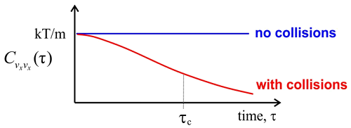
Let’s analyze a dilute gas of molecules which have a Maxwell–Boltzmann distribution of velocities. We focus on the component of the molecular velocity along the \(\hat{x}\) direction, \(x_v\). We know that the average velocity is \(\left\langle v _ {x} \right\rangle = 0\). The velocity correlation function is

\[C _ {v _ {x} v _ {x}} ( \tau ) = \left\langle v _ {x} ( \tau ) v _ {x} ( 0 ) \right\rangle \nonumber \]

From the equipartition principle the average translational energy is

\[\frac {1} {2} m \left\langle v _ {x}^{2} \right\rangle = k _ {B} T / 2 \nonumber\]

For time scales short compared to collisions between molecules, the velocity of any given molecule remains constant and unchanged, so the correlation function for the velocity is also unchanged at \(k_BT/m\). This non-interacting regime corresponds to the behavior of an ideal gas.

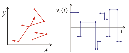
For any real gas, there will be collisions that randomize the direction and speed of the molecules, so that any molecule over a long enough time will sample the various velocities within the Maxwell–Boltzmann distribution. From the trajectory of x-velocities for a given molecule we can calculate \(C _ {v _ {x _ {x}}} ( \tau )\) using time-averaging. The correlation function will drop on with a correlation time \(\tau_c\), which is related to mean time between collisions. After enough collisions, the correlation with the initial velocity is lost and \(C _ {v _ {x _ {x}}} ( \tau )\) approaches \(\left\langle v _ {x}^{2} \right\rangle = 0\). Finally, we can determine the diffusion constant for the gas, which relates the time and mean square displacement of the molecules:

\[\left\langle x^{2} (t) \right\rangle = 2 D _ {x} t.\nonumber\]

From

\[D _ {x} = \int _ {0}^{\infty} d t \left\langle v _ {x} (t) v _ {x} ( 0 ) \right\rangle\nonumber\]

we have

\[D _ {x} = k _ {B} T \tau _ {c} / m\nonumber\]

In viscous fluids \(\tau _ {c} / m\) is called the mobility, \(\mu\).

Example \(\PageIndex{2}\): Dipole Moment Correlation Function

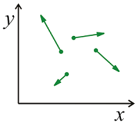
Now consider the correlation function for the dipole moment of a polar diatomic molecule in a dilute gas, \(\overline {\mu}\). For a rigid rotating object, we can decompose the dipole into a magnitude and a direction unit vector:

\[\overline {\mu} _ {i} = \mu _ {0} \cdot \hat {u}.\nonumber\]

We know that \(\langle \hat {\mu} \rangle = 0\) since all orientations of the gas phase molecules are equally probable. The correlation function is

\[\begin{align*} C _ {\mu \mu} (t) & = \langle \overline {\mu} (t) \overline {\mu} ( 0 ) \rangle \\[4pt] & = \left\langle \mu _ {0}^{2} \right\rangle \langle \hat {u} (t) \cdot \hat {u} ( 0 ) \rangle \end{align*}\]

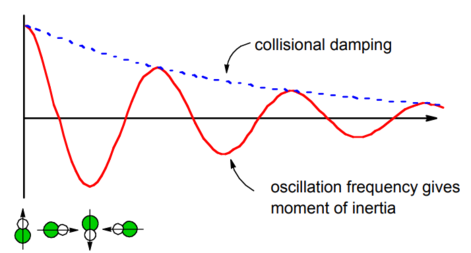
This correlation function projects the time-dependent orientation of the molecule onto the initial orientation. Free inertial rotational motion will lead to oscillations in the correlation function as the dipole spins. The oscillations in this correlation function can be related to the speed of rotation and thereby the molecule’s moment of inertia (discussed below). Any apparent damping in this correlation function would reflect the thermal distribution of angular velocities. In practice a real gas would also have the collisional damping effects described in Example \(\PageIndex{1}\) superimposed on this relaxation process.

Example \(\PageIndex{3}\): Harmonic Oscillator Correlation Function

The time-dependent motion of a harmonic vibrational mode is given by Newton’s law in terms of the acceleration and restoring force as \(m \ddot {q} = - \kappa q\) or \(\ddot {q} = - \omega^{2} q\) where the force constant is \(\kappa = m \omega^{2}\). We can write a common solution to this equation as

\[q (t) = q ( 0 ) \cos \omega t\nonumber\]

Furthermore, the equipartition theorem says that the equilibrium thermal energy in a harmonic vibrational mode is

\[\frac {1} {2} \kappa \left\langle q^{2} \right\rangle = \frac {k _ {B} T} {2}\nonumber\]

We therefore can write the correlation function for the harmonic vibrational coordinate as

\[\begin{align*} C _ {q q} (t) &= \langle q (t) q ( 0 ) \rangle \\[4pt] &= \left\langle q^{2} \right\rangle \cos \omega t \\[4pt] & = \frac {k _ {B} T} {\kappa} \cos \omega t \end{align*}\]