1.5: Numerically Solving the Schrödinger Equation

Often the bound potentials that we encounter are complex, and the time-independent Schrödinger equation will need to be evaluated numerically. There are two common numerical methods for solving for the eigenvalues and eigenfunctions of a potential. Both methods require truncating and discretizing a region of space that is normally spanned by an infinite dimensional Hilbert space. The Numerov method is a finite difference method that calculates the shape of the wavefunction by integrating step-by-step across along a grid. The DVR method makes use of a transformation between a finite discrete basis and the finite grid that spans the region of interest.

Figure \(\PageIndex{1}\): Selection and discretization of a space bounding the region for which the TISE will be solved numerically. A space of length \(L\) is discretized into \(N\) points separated by a spacing \(δx\) over which the potential varies slowly.

The Numerov Method

A one-dimensional Schrödinger equation for a particle in a potential can be numerically solved on a grid that discretizes the position variable using a finite difference method. The TISE is

\[[ T + V (x) ] \psi (x) = E \psi (x) \label{128}\]

with

\[T = - \dfrac {\hbar^{2}} {2 m} \dfrac {\partial^{2}} {\partial x^{2}},\]

which we can write as

\[\psi^{\prime \prime} (x) = - k^{2} (x) \psi (x) \label{129}\]

where

\[k^{2} (x) = \dfrac {2 m} {\hbar^{2}} [ E - V (x) ].\]

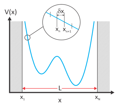
If we discretize the variable \(x\), choosing a grid spacing \(\delta x\) over which \(V\) varies slowly, we can use a three point finite difference to approximate the second derivative:

\[f _ {i}^{\prime \prime} \approx \dfrac {1} {\delta x^{2}} \left( f \left( x _ {i + 1} \right) - 2 f \left( x _ {i} \right) + f \left( x _ {i - 1} \right) \right) \label{130}\]

The discretized Schrödinger equation can then be written in the form

\[\psi \left( x _ {i + 1} \right) - 2 \psi \left( x _ {i} \right) + \psi \left( x _ {i - 1} \right) = - k^{2} \left( x _ {i} \right) \psi \left( x _ {i} \right) \label{131}\]

Using the equation for \(\psi \left( x _ {i + 1} \right)\), one can iteratively solve for the eigenfunction. In practice, you discretize over a range of space such that the highest and lowest values lie in a region where the potential is very high or forbidden. Splitting the space into N points, chose the first two values \(\psi \left( x _ {1} \right) = 0\) and \(\psi \left( x _ {2} \right)\)x to be a small positive or negative number, guess \(E\), and propagate iteratively to \(\psi \left( x _ {N} \right)\). A comparison of the wavefunctions obtained by propagating from \(x_1\) to \(x_N\) with that obtained propagating from \(x_N\) to \(x_1\) tells you how good your guess of \(E\) was.

The Numerov Method improves on Equation \ref{131} by taking account for the fourth derivative of the wavefunction \(\Psi^{( 4 )}\), leading to errors on the order \(O \left( \delta x^{6} \right)\). Equation \ref{130} becomes

\[f _ {i}^{\prime \prime} \approx \dfrac {1} {\delta x^{2}} \left( f \left( x _ {i + 1} \right) - 2 f \left( x _ {i} \right) + f \left( x _ {i - 1} \right) \right) - \dfrac {\delta x^{2}} {12} f _ {i}^{( 4 )} \label{132}\]

By differentiating Equation \ref{129} we know

\[\psi^{( 4 )} (x) = - \left( k^{2} (x) \psi (x) \right)^{\prime \prime}\]

and the discretized Schrödinger equation becomes

\[\left.\begin{aligned} \psi^{\prime \prime} \left( x _ {i} \right) & = \dfrac {1} {\delta x^{2}} \left( \psi \left( x _ {i + 1} \right) - 2 \psi \left( x _ {i} \right) + \psi \left( x _ {i - 1} \right) \right) + \\ & \dfrac {1} {12} \left( k^{2} \left( x _ {i + 1} \right) \psi \left( x _ {i + 1} \right) - 2 k^{2} \left( x _ {i + 1} \right) \psi \left( x _ {i} \right) + k^{2} \left( x _ {i + 1} \right) \psi \left( x _ {i - 1} \right) \right) \end{aligned} \right. \label{33}\]

This equation leads to the iterative solution for the wavefunction

\[\psi \left( x _ {i + 1} \right) = \dfrac{\psi \left( x _ {i} \right) \left( 2 + \dfrac {10 \delta x^{2}} {12} k^{2} \left( x _ {i} \right) \right) - \psi \left( x _ {i - 1} \right) \left( 1 - \dfrac {\delta x^{2}} {12} k^{2} \left( x _ {i - 1} \right) \right)}{1 - \dfrac {\delta x^{2}} {12} k^{2} \left( x _ {i + 1} \right)} \label{134}\]

Discrete Variable Representation (DVR)

Numerical solutions to the wavefunctions of a bound potential in the position representation require truncating and discretizing a region of space that is normally spanned by an infinite dimensional Hilbert space. The DVR approach uses a real space basis set whose eigenstates \(\varphi _ {i} (x)\) we know and that span the space of interest—for instance harmonic oscillator wavefunctions—to express the eigenstates of a Hamiltonian in a grid basis (\(\theta _ {j}\)) that is meant to approximate the real space continuous basis \(\delta (x)\). The two basis sets, which we term the eigenbasis (\(\varphi\)) and grid basis (\(\theta\)), will be connected through a unitary transformation

\(\Phi^{\dagger} \varphi (x) = \theta (x) \label{135}\) \(\Phi \theta (x) = \varphi (x)\)

For \(N\) discrete points in the grid basis, there will be \(N\) eigenvectors in the eigenbasis, allowing the properties of projection and completeness will hold in both bases. Wavefunctions can be obtained by constructing the Hamiltonian in the eigenbasis,

\(H = T ( \hat {p} ) + V ( \hat {x} ),\) transforming to the DVR basis, \(H^{D V R} = \Phi H \Phi,\) and then diagonalizing.

Here we will discuss a version of DVR in which the grid basis is set up to mirror the continuous \(| \mathcal {X} \rangle\) eigenbasis. We begin by choosing the range of \(x\) that contain the bound states of interest and discretizing these into \(N\) points (\(x_i\)) equally spaced by \(δx\). We assume that the DVR basis functions \(\theta _ {j} \left( x _ {i} \right)\) resemble the infinite dimensional position basis

\[\theta _ {j} \left( x _ {i} \right) = \sqrt {\Delta x} \delta _ {i j} \label{136}\]

Our truncation is enabled using a projection operator in the reduced space

\[P _ {N} = \sum _ {i = 1}^{N} | \theta _ {i} \rangle \langle \theta _ {i} | \approx 1 \label{137}\]

which is valid for appropriately high \(N\). The complete Hamiltonian can be expressed in the DVR basis DVR

\[H^{D V R} = T^{D V R} + V^{D V R}.\]

For the potential energy, since \(\left\{\theta _ {i} \right\}\) is localized with \(\left\langle \theta _ {i} | \theta _ {j} \right\rangle = \delta _ {i j}\), we make the DVR approximation, which casts \(V^{DVR}\) into a diagonal form that is equal to the potential energy evaluated at the grid point:

\[V _ {i j}^{D V R} = \left\langle \theta _ {i} | V ( \hat {x} ) | \theta _ {j} \right\rangle \approx V \left( x _ {i} \right) \delta _ {i j} \label{138}\]

This comes from approximating the transformation as \(\Phi V ( \hat {x} ) \Phi^{\dagger} \approx V \left( \Phi \hat {x} \Phi^{\dagger} \right) . \)

For the kinetic energy matrix elements \(\left\langle \theta _ {i} | T ( \hat {p} ) | \theta _ {j} \right\rangle\), we need to evaluate second derivatives between different grid points. Fortunately, Colbert and Miller have simplified this process by finding an analytical form for the \(T^{DVR}\) matrix for a uniformly gridded box with a grid spacing of \(∆x\).

\[T _ {i j}^{\mathrm {DVR}} = \dfrac {\hbar^{2} ( - 1 )^{i - j}} {2 m \Delta x^{2}} \left\{\begin{array} {c c} {\pi^{2} / 3} & {i = j} \\ {2 / ( i - j )^{2}} & {i \neq j} \end{array} \right\} \label{139}\]

This comes from a Fourier expansion in a uniformly gridded box. Naturally this looks oscillatory in \(x\) at period of \(δx\). Expression becomes exact in the limit of \(N \rightarrow \infty\) or \(\Delta x \rightarrow 0\). The numerical routine becomes simple and efficient. We construct a Hamiltonian filling with matrix elements whose potential and kinetic energy contributions are given by Equations \ref{138} and \ref{139}. Then we diagonalize \(H^{DVR}\), from which we obtain \(N\) eigenvalues and the \(N\) corresponding eigenfunctions.

References

1. I. N. Levine, Quantum Chemistry, 5th ed. (Prentice Hall, Englewood Cliffs, NJ, 2000).
2. J. C. Light and T. Carrington, "Discrete-Variable Representations and Their Utilization" in Advances in Chemical Physics (John Wiley & Sons, Inc., 2007), pp. 263-310;
3. D. J. Tannor, Introduction to Quantum Mechanics: A Time-Dependent Perspective. (University Science Books, Sausilito, CA, 2007).
4. D. T. Colbert and W. H. Miller, A Novel Discrete Variable Representation for Quantum Mechanical Reactive Scattering Via the S‐Matrix Kohn Method, J. Chem. Phys. 96, 1982-1991 (1992).