1.3: Basic Quantum Mechanical Models

This section summarizes the results that emerge for common models for quantum mechanical objects. These form the starting point for describing the motion of electrons and the translational, rotational, and vibrational motions for molecules. Thus they are the basis for developing intuition about more complex problems.

Waves

Waves form the basis for our quantum mechanical description of matter. Waves describe the oscillatory amplitude of matter and fields in time and space, and can take a number of forms. The simplest form we will use is plane waves, which can be written as

\[\psi ( \mathbf {r} , t ) = \mathbf {A} \exp [ i \mathbf {k} \cdot \mathbf {r} - \mathbf {i} \omega t ] \label{43}\]

The angular frequency \(ω\) describes the oscillations in time and is related to the number of cycles per second through \(ν = ω/2π\). The wave amplitude also varies in space as determined by the wavevector \(\mathbf {k}\), where the number of cycles per unit distance (wavelength) is \(λ = ω/k\). Thus the wave propagates in time and space along a direction \(\mathbf {k}\) with a vector amplitude A with a phase velocity \(vϕ = νλ\).

Free Particles

For a free particle of mass \(m\) in one dimension, the Hamiltonian only reflects the kinetic energy of the particle

\[\hat {H} = \hat {T} = \frac {\hat {p}^{2}} {2 m} \label{44}\]

Judging from the functional form of the momentum operator, we assume that the wavefunctions will have the form of plane waves

\[\psi (x) = A e^{i k x} \label{45}\]

Inserting this expression into the TISE, eq. (1.1.6), we find that

\[k = \sqrt {\frac {2 m E} {\hbar^{2}}} \label{46}\]

and set \(A = 1 / \sqrt {2 \pi}\). Now, since we know that \(E = p^{2} / 2 m\), we can write

\[k = \frac {p} {\hbar} \label{47}\]

\(k\) is the wavevector, which we equate with the momentum of the particle.

Free particle plane waves \(\psi _ {k} (x)\) form a complete and continuous basis set with which to describe the wavefunction. Note that the eigenfunctions, Equation (\ref{45}), are oscillatory over all space. Thus describing a plane wave allows one to exactly specify the wavevector or momentum of the particle, but one cannot localize it to any point in space. In this form, the free particle is not observable because its wavefunction extends infinitely and cannot be normalized. An observation, however, taking an expectation value of a Hermitian operator will collapse this wavefunction to yield an average momentum of the particle with a corresponding uncertainty relationship to its position.

Bound particles

Particle-in-a-Box

The minimal model for translational motion of a particle that is confined in space is given by the particle-in-a-box. For the case of a particle confined in one dimension in a box of length L with impenetrable walls, we define the Hamiltonian as

\[\hat {H} = \frac {\hat {p}^{2}} {2 m} + V (x) \label{48}\]

\[V (x) = \left\{\begin{array} {l l} {0} & {0 < x < L _ {x}} \\ {\infty} & {\text {otherwise}} \end{array} \right. \label{49}\]

The boundary conditions require that the particle cannot have any probability of being within the wall, so the wavefunction should vanish at \(x = 0\) and \(L_x\), as with standing waves. We therefore assume a solution in the form of a sine function. The properly normalized eigenfunctions are

\[\psi _ {n} = \sqrt {\frac {2} {L}} \sin \frac {n \pi x} {L} \quad n = 1,2,3 \dots \label{50}\]

Here \(n\) are the integer quantum numbers that describe the harmonics of the fundamental frequency \(\pi/L\) whose oscillations will fit into the box while obeying the boundary conditions. We see that any state of the particle-in-a-box can be expressed in a Fourier series. On inserting Equation \ref{50} into the time-independent Schrödinger equation, we find the energy eigenvalues

\[E _ {n} = \frac {n^{2} \pi^{2} h^{2}} {2 m L^{2}} \label{51}\]

Note that the spacing between adjacent energy levels grows as \(n(n+1)\). This model is readily extended to a three-dimensional box by separating the box into \(x\), \(y\), and \(z\) coordinates. Then

\[\hat {H} = \hat {H} _ {x} + \hat {H} _ {y} + \hat {H} _ {z} \label{52}\]

in which each term is specified as Equation \ref{48}. Since \(\hat {H} _ {x}\), \(\hat {H} _ {y}\), \(\hat {H} _ {z}\) commute, each dimension is separable from the others. Then we find

\[\psi ( x , y , z ) = \psi _ {x} \psi _ {y} \psi _ {z} \label{53}\]

and

\[E _ {x , y , z} = E _ {x} + E _ {y} + E _ {z} \label{54}\]

which follow the definitions given in Equation \ref{50} and \ref{51} above. The state of the system is now specified by three quantum numbers with positive integer values: \(n_x\), \(n_y\), \(n_z\)

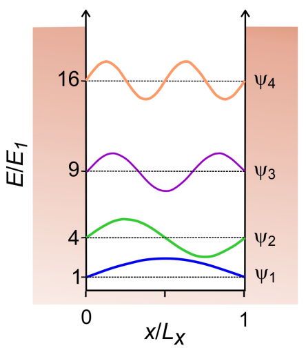
Figure 1. Particle-in-a-box potential wavefunctions that are plotted superimposed on their corresponding energy levels.

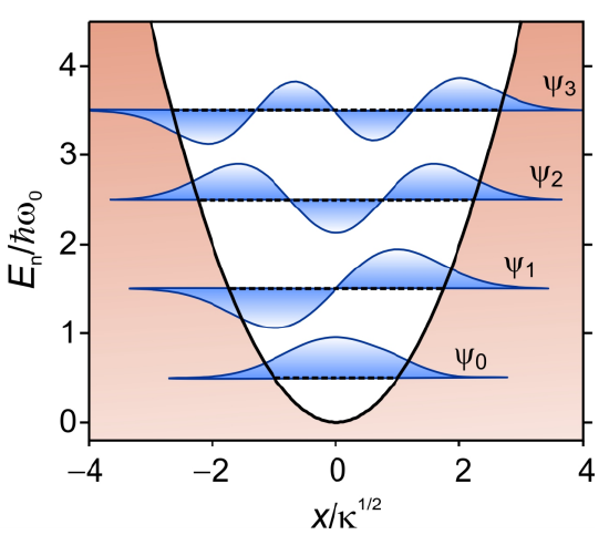
Figure 2. Harmonic oscillator potential showing wavefunctions that are superimposed on their corresponding energy levels.

Harmonic Oscillator

The harmonic oscillator Hamiltonian refers to a particle confined to a parabolic, or harmonic, potential. We will use it to represent vibrational motion in molecules, but it also becomes a general framework for understanding all bosons. For a classical particle bound in a one-dimensional potential, the potential near the minimum \(x_0\) can be expanded as

\[V (x) = V \left( x _ {0} \right) + \left( \frac {\partial V} {\partial x} \right) _ {x = x _ {0}} \left( x - x _ {0} \right) + \frac {1} {2} \left( \frac {\partial V^{2}} {\partial x^{2}} \right) _ {x = x _ {0}} \left( x - x _ {0} \right)^{2} + \cdots \label{55}\]

Setting \(x_0\) to 0, the leading term with a dependence on \(x\) is the second-order (harmonic) term \(V = - \mathrm {K} x^{2} / 2\), where the force constant

\[\kappa = - \left( \partial^{2} V / \partial x^{2} \right) _ {x = 0}.\]

The classical Hamiltonian for a particle of mass \(m\) confined to this potential is

\[H = \frac {p^{2}} {2 m} + \frac {1} {2} \kappa x^{2} \label{56}\]

Noting that the force constant and frequency of oscillation are related by

\[\kappa = m \omega _ {0}^{2},\]

we can substitute operators for \(p\) and \(x\) in Equation \ref{56} to obtain the quantum Hamiltonian

\[\hat {H} = - \frac {1} {2} \frac {\hbar^{2}} {m} \frac {\partial^{2}} {\partial x^{2}} + \frac {1} {2} m \omega _ {0}^{2} \hat {x}^{2} \label{57}\]

We will also make use of reduced mass-weighted coordinates defined as

\[p = \sqrt {\frac {2} {m \hbar \omega _ {0}}} \hat {p}\label{58A}\]

\[x = \sqrt {\frac {m \omega _ {0}} {2 \hbar}} \hat {x} \label{58B}\]

for which the Hamiltonian can be written as

\[\hat {H} = \hbar \omega _ {0} \left( p^{2} + q^{2} \right) \label{59}\]

The eigenstates for the Harmonic oscillator are expressed in terms of Hermite polynomials

\[\psi _ {n} (x) = \sqrt {\frac {\alpha} {2^{n} \sqrt {\pi} n !}} e^{- \alpha^{2} x^{2} / 2} \mathcal {H} _ {n} ( \alpha x ) \label{60}\]

where \(\alpha=\sqrt{m \omega_{0} / \hbar}\) and the Hermite polynomials are obtained from

\[\mathcal {H} _ {n} (x) = ( - 1 )^{n} e^{x^{2}} \frac {d^{n}} {d x^{n}} e^{- x^{2}} \label{61}\]

The corresponding energy eigenvalues are equally spaced in units of the vibrational quantum \(\hbar \omega _ {0} \) above the zero-point energy \(\hbar \omega _ {0} / 2\).

\(E_{n}=\hbar \omega_{0}\left(n+\frac{1}{2}\right) \quad n=0,1,2 \ldots \label{62}\)

Raising and Lowering Operators for Harmonic Oscillators

From a practical point of view, it will be most useful for us to work problems involving harmonic oscillators in terms of raising and lower operators (also known as creation and annihilation operators, or ladder operators). We define these as

\[\hat {a} = \sqrt {\frac {2 \hbar} {m \omega _ {0}}} \left( \hat {x} + \frac {i} {m \omega _ {0}} \hat {p} \right) \label{63}\]

\[\hat {a}^{\dagger} = \sqrt {\frac {2 \hbar} {m \omega _ {0}}} \left( \hat {x} - \frac {i} {m \omega _ {0}} \hat {p} \right) \label{64}\]

Note \(a\) and \(a^†\) operators are Hermitian conjugates of one another. These operators get their name from their action on the harmonic oscillator wavefunctions, which is to lower or raise the state of the system:

\[\hat {a} | n \rangle = \sqrt {n} | n - 1 \rangle \label{65}\]

and

\[\hat {a}^{\dagger} | n \rangle = \sqrt {n + 1} | n + 1 \rangle\]

Then we find that the position and momentum operators are

\[\hat {x} = \sqrt {\frac {\hbar} {2 m \omega _ {0}}} \left( \hat {a}^{\dagger} + \hat {a} \right) \label{66}\]

\[\hat {p} = i \sqrt {\frac {m \hbar \omega _ {0}} {2}} \left( \hat {a}^{\dagger} - \hat {a} \right) \label{67}\]

When we substitute these ladder operators for the position and momentum operators—known as second quantization—the Hamiltonian becomes

\[\hat {H} = \hbar \omega _ {0} \left( \hat {n} + \frac {1} {2} \right) \label{68}\]

The number operator is defined as \(\hat {n} = \hat {a}^{\dagger} \hat {a}\) and returns the state of the system: \(\hat {n} = \hat {a}^{\dagger} \hat {a}\). The energy eigenvalues satisfying \(\hat {H} | n \rangle = E _ {n} | n \rangle\) are given by Equation \ref{62). Since the quantum numbers cannot be negative, we assert a boundary condition \(a | 0 \rangle = 0\), where \(0\) refers to the null vector. The harmonic oscillator Hamiltonian expressed in raising and lowering operators, together with its commutation relationship

\[\left[ a , a^{\dagger} \right] = 1 \label{69}\]

is used as a general representation of all bosons, which for our purposes includes vibrations and photons.

Properties of raising and lower operators

\(a\) and \(a^†\) a operators are Hermitian conjugates of one another.

\[a a^{\dagger} + a^{\dagger} a = a^{\dagger} a + \frac {1} {2} \label{70}\]

\[\left[ a , a^{\dagger} \right] = 1 \label{71}\]

\[[ a , a ] = 0 \left[ a^{\dagger} , a^{\dagger} \right] = 0 \label{72}\]

\[\left[ a , \left( a^{\dagger} \right)^{n} \right] = n \left( a^{\dagger} \right)^{n - 1} \label{73}\]

\[\left[ a^{\dagger} , a^{n} \right] = - n a^{n - 1} \label{74}\]

\[| n \rangle = \frac {1} {\sqrt {n !}} \left( a^{\dagger} \right)^{n} | 0 \rangle \label{75}\]

Morse Oscillator

The Morse oscillator is a model for a particle in a one-dimensional anharmonic potential energy surface with a dissociative limit at infinite displacement. It is commonly used for describing the spectroscopy of diatomic molecules and anharmonic vibrational dynamics, and most of its properties can be expressed through analytical expressions.3 The Morse potential is

\[V (x) = D _ {e} \left[ 1 - e^{- \alpha x} \right]^{2} \label{76}\]

where \(x = \left( r - r _ {0} \right)\). \(D_e\) sets the depth of the energy minimum at \(r = r_0\) relative to the dissociation limit as \(r → ∞\), and α sets the curvature of the potential. If we expand \(V\) in powers of \(x\) as described in Equation \ref{55}

\[V (x) \approx \frac {1} {2} \kappa x^{2} + \frac {1} {6} g x^{3} + \frac {1} {24} h x^{4} + \cdots \label{77}\]

we find that the harmonic, cubic, and quartic expansion coefficients are

\[\kappa = 2 D _ {e} \alpha^{2},\]

\[g = - 6 D _ {e} \alpha^{3},\]

and \[h = 14 D _ {e} \alpha^{4}.\]

The Morse oscillator Hamiltonian for a diatomic molecule of reduced mass mR bound by this potential is

\[H = \frac {p^{2}} {2 m _ {R}} + V (x) \label{78}\]

and has the eigenvalues

\[E _ {n} = \hbar \omega _ {0} \left[ \left( n + \frac {1} {2} \right) - x _ {e} \left( n + \frac {1} {2} \right)^{2} \right] \label{79}\]

Here \(\omega _ {0} = \sqrt {2 D _ {e} \alpha^{2} / m _ {R}}\) is the fundamental frequency and \(x _ {e} = \hbar \omega _ {0} / 4 D _ {e}\) is the anharmonic constant. Similar to the harmonic oscillator, the frequency \(\omega _ {0} = \sqrt {\kappa / m _ {R}}\). The anharmonic constant e x is commonly seen in the spectroscopy expression for the anharmonic vibrational energy levels

\[G ( v ) = \omega _ {e} \left( v + \frac {1} {2} \right) - \omega _ {e} x _ {e} \left( v + \frac {1} {2} \right)^{2} + \omega _ {e} y _ {e} \left( v + \frac {1} {2} \right)^{3} + \cdots \label{80}\]

From Equation \ref{79}, the ground state (or zero-point) energy is

\[E _ {0} = \frac {1} {2} \hbar \omega _ {0} \left( 1 - \frac {1} {2} x _ {e} \right) \label{81}\]

So the dissociation energy for the Morse potential is given by \(D_{0}=D_{e}-E_{0}\). The transition energies are

\[E _ {n} - E _ {m} = \hbar \omega _ {0} ( n - m ) \left[ 1 - x _ {e} \left( n + m + \frac {1} {2} \right) \right] \label{82}\]

The proper harmonic expressions are obtained from the corresponding Morse oscillator expressions by setting \(D _ {e} \rightarrow \infty\) or \(x _ {e} \rightarrow 0\).

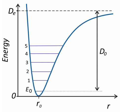
Figure 3. Shape of the Morse potential illustrating the first six energy eigenvalues.

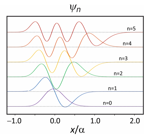
Figure 4. First six eigenfunctions of the Morse oscillator potential.

The wavefunctions for the Morse oscillator can also be expressed analytically in terms of associated Laguerre polynomials \(\mathcal {L} _ {n}^{\prime} ( z )\)

\[\psi _ {n} = N _ {n} e^{- z / 2} z^{b / 2} \mathcal {L} _ {n}^{b} ( z ) \label{83}\]

where \(N_{n}=[\alpha \cdot b \cdot n ! / \Gamma(k-n)]^{1 / 2}\), \(z=k \exp [-\alpha q], b=k-2 n-1\), and \(k=4 D_{e} / \hbar \omega_{0}\). These expressions and those for matrix elements in \(q, q^{2}, \mathrm{e}^{-\alpha q}, \text {and} q \mathrm{e}^{-\alpha q}\) have been given by Vasan and Cross.

Angular momentum

Angular Momentum Operators

To describe quantum mechanical rotation or orbital motion, one has to quantize angular momentum. The total orbital angular momentum operator is defined as

\[\hat{L}=\hat{r} \times \hat{p}=i \hbar(\hat{r} \times \nabla)\]

It has three components \(\left(\hat{L}_{x}, \hat{L}_{y}, \hat{L}_{z}\right)\) that generate rotation about the x, y, or z axis, and whose magnitude is given by

\(\hat{L}^{2}=\hat{L}_{x}^{2}+\hat{L}_{y}^{2}+\hat{L}_{z}^{2}\). The angular momentum operators follow the commutation relationships

\[\left[ H , L _ {z} \right] = 0 \label{85A}\]

\[\left[ H , L^{2} \right] = 0 \label{85B}\]

\[\left[ L _ {x} , L _ {y} \right] = i \hbar L _ {z} \label{86}\]

(In Equation \ref{86} the \(x\), \(y\), \(z\) indices can be cyclically permuted.) There is an eigenbasis common to \(H\) and \(L^2\) and one of the \(L_i\), which we take to be \(L_z\). The eigenvalues for the orbital angular momentum operator L and z-projection of the angular momentum Lz are

\[L^{2} | \ell m \rangle = \hbar^{2} \ell ( \ell + 1 ) | \ell m \rangle \quad \ell = 0,1,2 \ldots \label{87}\]

\[L _ {z} | \ell m \rangle = \hbar m | \ell m \rangle \quad m = 0 , \pm 1 , \pm 2 \ldots \pm \ell \label{88}\]

where the eigenstates \(| \ell m \rangle\) are labeled by the orbital angular momentum quantum number \(\ell\), and the magnetic quantum number, \(m\).

Similar to the strategy used for the harmonic oscillator, we can also define raising and lowering operators for the total angular momentum,

\[\hat {L} _ {\pm} = \hat {L} _ {i} \pm \mathrm {i} \hat {L} _ {y} \label{89}\]

which follow the commutation relations \(\left[ \hat {L}^{2} , \hat {L} _ {\pm} \right] = 0\) and \(\left[ \hat {L} _ {z} , \hat {L} _ {\pm} \right] = \pm \hbar \hat {L} _ {\pm}\), and satisfy the eigenvalue equation

\[\hat {L} _ {\pm} | \ell m \rangle = A _ {\ell , m} | \ell m \rangle \label{90}\]

\[A _ {\ell , m} = \hbar [ \ell ( \ell + 1 ) - m ( m \pm 1 ) ]^{1 / 2}\]

Spherically Symmetric Potential

Let’s examine the role of angular momentum for the case of a particle experiencing a spherically symmetric potential V(r) such as the hydrogen atom, 3D isotropic harmonic oscillator, and free particles or molecules. For a particle with mass \(m_{R}\), the Hamiltonian is

\[\hat{H}=-\frac{\hbar^{2}}{2 m} \nabla^{2}+V(r) \label{91}\]

Writing the kinetic energy operator in spherical coordinates,

\[-\frac{\hbar^{2}}{2 m} \nabla^{2}=-\frac{\hbar^{2}}{2 m}\left(\frac{1}{r^{2}} \frac{\partial}{\partial r} r^{2} \frac{\partial}{\partial r}-\frac{1}{r^{2}} L^{2}\right) \label{92}\]

where the square of the total angular momentum is

\[L^{2}=-\frac{1}{\sin \theta}\left(\frac{1}{\sin \theta} \frac{\partial^{2}}{\partial \phi^{2}}+\frac{\partial}{\partial \theta} \sin \theta \frac{\partial}{\partial \theta}\right) \label{93}\]

We note that this representation separates the radial dependence in the Hamiltonian from the angular part. We therefore expect that the overall wavefunction can be written as a product of a radial and an angular part in the form

\[\psi(r, \theta, \phi)=R(r) Y(\theta, \phi) \label{94}\]

Substituting this into the TISE, we find that we solve for the orientational and radial wavefunctions separately. Considering solutions first to the angular part, we note that the potential is only a function of r, and only need to consider the angular momentum. This leads to the identities in eqs. (\ref{87}) and (\ref{88}), and reveals that the \(|\ell m\rangle\) wavefunctions projected onto spherical coordinates are represented by the spherical harmonics

\[Y_{\ell}^{m}(\theta, \phi)=N_{t m}^{Y} P_{\ell}^{|m|}(\cos \theta) \mathrm{e}^{i m \phi} \label{95}\]

\(P_{\ell}^{m}\) are the associated Legendre polynomials and the normalization factor is

\[N_{(m}^{Y}=(-1)^{(m+\mid m) / 2} i^{\ell}\left[\frac{2 \ell+1}{4 \pi} \frac{(\ell-|m|) !}{(\ell+|m|) !}\right]^{1 / 2}\]

The angular components of the wavefunction are common to all eigenstates of spherically symmetric potentials. In chemistry, it is common to use real angular wavefunctions instead of the complex form in eq. (\ref{95}). These are constructed from the linear combinations \(Y_{\mathrm{n}, z} \pm Y_{\mathrm{n},-\ell}\).

Substituting eq. (\ref{92}) and eq. (\ref{87}) into eq. (\ref{91}) leads to a new Hamiltonian that can be inserted into the Schrödinger equation. This can be solved as a purely radial problem for a given value of \(l\). It is convenient to define the radial distribution function \(\chi(r)=r R(r)\), which allows the TISE to be rewritten as

\[\left(-\frac{\hbar^{2}}{2 m} \frac{\partial^{2}}{\partial r^{2}}+U(r, \ell)\right) \chi=E \chi \label{96}\]

U plays the role of an effective potential

\[U(r, \ell)=V(r)+\frac{\hbar^{2}}{2 m r^{2}} \ell(\ell+1) \label{97}\]

Equation (\ref{96}) is known as the radial wave equation. It looks like the TISE for a one-dimensional problem in r, where we could solve this equation for each value of \(\ell\). Note U has a barrier due to centrifugal kinetic energy that scales as \(r^{-2} \text {for} \ell>0\).

The wavefunctions defined in eq. (\ref{94}) are normalized such that

\[\int|\psi|^{2} d \Omega=1 \label{98}\]

where

\[\int d \Omega \equiv \int_{0}^{\infty} r^{2} d r \int_{0}^{\pi} \sin \theta d \theta \int_{0}^{2 \pi} d \phi \label{99}\]

If we restrict the integration to be over all angles, we find that the probability of finding a particle between a distance r and \(r+d r \text {is} P(r)=4 \pi r^{2}|R(r)|^{2}=4 \pi|\chi(r)|^{2}\).

To this point the treatment of orbital angular momentum is identical for any spherically symmetric potential. Now we must consider the specific form of the potential; for instance in the case of the isotropic harmonic oscillator, \(U(r)=1 / 2 \kappa r^{2}\). In the case of a free particle, we substitute \(V(r)=0 \text {in eq.}(\ref{97})\) and find that the radial solutions can be written in terms of spherical Bessel functions, \(j_{\ell}\). Then the solutions to the full wavefunction for the free particle can be written as

\[\Psi(r, \theta, \phi)=j_{\ell}(\mathrm{k} r) Y_{\ell}^{m}(\theta, \phi) \label{100}\]

where the wavevector k is defined as in eq. (\ref{46}).

Hydrogen Atom

For a hydrogen-like atom, a single electron of charge e interacts with a nucleus of charge \(Ze\) under the influence of a Coulomb potential

\[V_{H}(r)=-\frac{Z e^{2}}{4 \pi \epsilon_{0}} \frac{1}{r} \label{101}\]

We can simplify the expression by defining atomic units for distance and energy. The Bohr radius is defined as

\[a_{0}=4 \pi \varepsilon_{0} \frac{\hbar^{2}}{m_{e} e^{2}}=5.2918 \times 10^{-11} \mathrm{~m} \label{102}\]

and the Hartree is

\[\mathcal{E}_{H}=\frac{1}{4 \pi \varepsilon_{0}} \frac{e^{2}}{a_{0}}=4.3598 \times 10^{-18} J=27.2 \mathrm{eV} \label{103}\]

Written in terms of atomic units, we can see from eq. (\ref{103}) that eq. (\ref{101}) becomes \(\left(V / \mathcal{E}_{H}\right)=-Z /\left(r / a_{0}\right)\). Thus the conversion effectively sets the SI variables \(m_{\mathrm{e}}=e=\left(4 \pi \varepsilon_{0}\right)^{-1}=\hbar = 1\). Then the radial wave equation is

\[\frac{\partial^{2} \chi}{\partial r^{2}}+\left(\frac{2 Z}{r}-\frac{\ell(\ell+1)}{r^{2}}\right) \chi=2 E \chi \label{104}\]

The effective potential within the parentheses in eq. (\ref{104}) is shown in Figure 5 for varying \(\ell\). Solutions to the radial wavefunction for the hydrogen atom take the form

\[R_{n \ell}(r)=N_{n \ell}^{R} \rho^{\ell} \mathcal{L}_{n+\ell}^{2 \ell+1}(\rho) e^{-\rho / 2} \label{105}\]

where the reduced radius \(\rho=2 r / n a_{0} \text {and} \mathcal{L}_{k}^{\alpha}(z)\) are the associated Laguerre polynomials. The primary quantum number takes on integer values \(n=1,2,3 \ldots, \text {and} \ell\) is constrained such that \(\ell= 0,1,2 \ldots n-1\). The radial normalization factor in eq. (\ref{105}) is

\[N_{n \ell}^{R}=-\frac{2}{n^{3} a_{0}^{3 / 2}}\left[\frac{(\mathrm{n}-\ell-1) !}{[(n+1) !]^{3}}\right]^{1 / 2} \label{106}\]

The energy eigenvalues are

\[E_{n}=-\frac{Z^{2}}{2 n^{2}} \mathcal{E}_{H} \label{107}\]

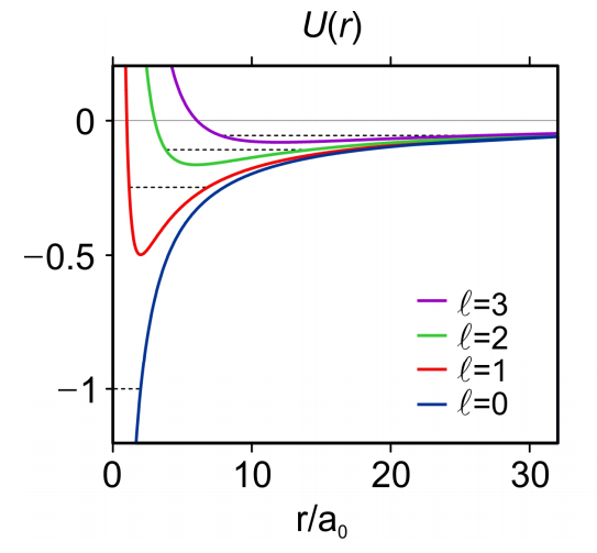
Figure 5. The radial effective potential, \(U_{e f f}(\rho)\)

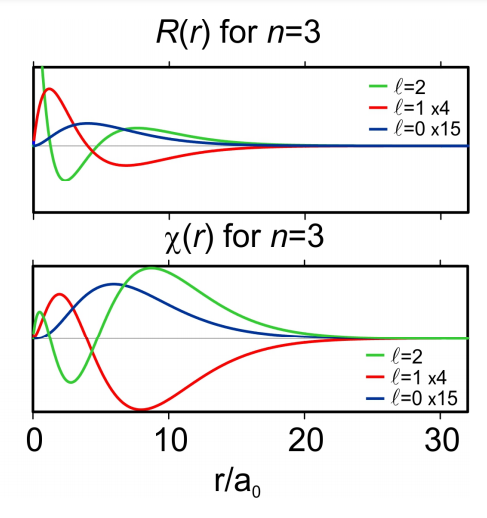
Figure 6. Radial probability density R and radial distribution function \(\chi=r R\).

Electron Spin

In describing electronic wavefunctions, the electron spin also results in a contribution to the total angular momentum, and results in a spin contribution to the wavefunction. The electron spin angular momentum S and its z-projection are quantized as

\[S^{2}\left|s m_{s}\right\rangle=\hbar^{2} s(s+1)\left|s m_{s}\right\rangle \quad s=0,1 / 2,1,3 / 2,2 \ldots \label{108}\]

\[S_{z}\left|s m_{s}\right\rangle=\hbar m_{s}\left|s m_{s}\right\rangle \quad m_{s}=-s,-s+1, \ldots, s \label{109}\]

where the electron spin eigenstates \(\left|s m_{s}\right\rangle\) are labeled by the electron spin angular momentum quantum number s and the spin magnetic quantum number \(m s\). The number of values of \(S_{z}\) is \(2 s+1\) and is referred to as the spin multiplicity. As fermions, electrons have half-integer spin, and each unpaired electron contributes \(1 / 2\) to the electron spin quantum number s. A single unpaired electron has \(s=1 / 2, \text {for which} m_{s}=\pm 1 / 2\) corresponding to spin-up and spin-down configurations. For multi-electron systems, the spin is calculated as the vector sum of spins, essentially \(1 / 2\) times the number of unpaired electrons.

The resulting total angular momentum for an electron is \(J=L+S\). J has associated with it the total angular momentum quantum number \(j\), which takes on values of \(j=|\ell-s|,|\ell-s|+1, \ldots \ell+s\). The additive nature of the orbital and spin contributions to the angular momentum leads to a total electronic wavefunction that is a product of spatial and spin wavefunctions.

\[\Psi_{\text {tot}}=\Psi(r, \theta, \phi)\left|s m_{s}\right\rangle \label{110}\]

Thus the state of an electron can be specified by four quantum numbers \(\Psi_{t o t}=\left|n \ell m_{\ell} m_{s}\right\rangle\).

Rigid Rotor

In the case of a freely spinning anisotropic molecule, the total angular momentum J is obtained from the sum of the orbital angular momentum L and spin angular momentum S for the molecular constituents: \(J=L+S, \text {where} L=\sum_{i} L_{i} \text {and} S=\sum_{i} S_{i}\). The case of the rigid rotor refers to the minimal model for the rotational quantum states of a freely spinning object that has cylindrical symmetry and no magnetic spin. Then, the Hamiltonian is given by the rotational kinetic energy

\[H_{r o t}=\frac{\hat{J}^{2}}{2 I} \label{111}\]

I is the moment of inertia about the principle axis of rotation. The eigenfunctions for this Hamiltonian are spherical harmonics \(Y_{J, M}(\theta, \phi)\)

\[\begin{array}{ll}
\hat{J}^{2}\left|Y_{J, M}\right\rangle=\hbar^{2} J(J+1)\left|Y_{J, M}\right\rangle & J=0,1,2 \ldots \\
\hat{J}_{z}\left|Y_{J, M}\right\rangle=M \hbar\left|Y_{J, M}\right\rangle & M=-J,-J+1, \ldots, J
\end{array} \label{112}\]

J is the rotational quantum number. M is its projection onto the z axis. The energy eigenvalues for \(H_{\text {rot}}\) are

\[E_{J, M}=\bar{B} J(J+1) \label{113}\]

where the rotational constant is

\[\bar{B}=\frac{\hbar^{2}}{2 I} \label{114}\]

More commonly, \(\bar{B}\) is given in units of \(c m^{-1} \text {using} \bar{B}=h / 8 \pi^{2} I c\).