
1.27: Spectroscopy - Interaction of Atoms and Molecules with Light
- Page ID
- 9350

In our final application of group theory, we will investigate the way in which symmetry considerations influence the interaction of light with matter. We have already used group theory to learn about the molecular orbitals in a molecule. In this section we will show that it may also be used to predict which electronic states may be accessed by absorption of a photon. We may also use group theory to investigate how light may be used to excite the various vibrational modes of a polyatomic molecule.
Last year, you were introduced to spectroscopy in the context of electronic transitions in atoms. You learned that a photon of the appropriate energy is able to excite an electronic transition in an atom, subject to the following selection rules:
\[\begin{array}{rcl} \Delta n & = & \text{integer} \\ \Delta l & = & \pm 1 \\ \Delta L & = & 0, \pm 1 \\ \Delta S & = & 0 \\ \Delta J & = & 0, \pm 1; J=0 \not \leftrightarrow J=0 \end{array} \tag{27.1}\]
What you may not have learned is where these selection rules come from. In general, different types of spectroscopic transition obey different selection rules. The transitions you have come across so far involve changing the electronic state of an atom, and involve absorption of a photon in the UV or visible part of the electromagnetic spectrum. There are analogous electronic transitions in molecules, which we will consider in more detail shortly. Absorption of a photon in the infrared (IR) region of the spectrum leads to vibrational excitation in molecules, while photons in the microwave (MW) region produce rotational excitation. Each type of excitation obeys its own selection rules, but the general procedure for determining the selection rules is the same in all cases. It is simply to determine the conditions under which the probability of a transition is not identically zero.
The first step in understanding the origins of selection rules must therefore be to learn how transition probabilities are calculated. This requires some quantum mechanics.
Last year, you learned about operators, eigenvalues and eigenfunctions in quantum mechanics. You know that if a function is an eigenfunction of a particular operator, then operating on the eigenfunction with the operator will return the observable associated with that state, known as the eigenvalue (i.e. \(\hat{A} \Psi = a \Psi\)). What you may not know is that operating on a function that is NOT an eigenfunction of the operator leads to a change in state of the system. In the transitions we will be considering, the molecule interacts with the electric field of the light (as opposed to NMR spectroscopy, in which the nuclei interact with the magnetic field of the electromagnetic radiation). These transitions are called electric dipole transitions, and the operator we are interested in is the electric dipole operator, usually given the symbol \(\hat{\boldsymbol{\mu}}\), which describes the electric field of the light.
If we start in some initial state \(\Psi_i\), operating on this state with \(\hat{\boldsymbol{\mu}}\) gives a new state, \(\Psi = \hat{\boldsymbol{\mu}} \Psi\). If we want to know the probability of ending up in some particular final state \(\Psi_f\), the probability amplitude is simply given by the overlap integral between \(\Psi\) and \(\Psi_f\). This probability amplitude is called the transition dipole moment, and is given the symbol \(\boldsymbol{\mu}_{fi}\)..
\[\hat{\boldsymbol{\mu}}_{fi} = \langle\Psi_f | \Psi\rangle = \langle\Psi_f | \hat{\boldsymbol{\mu}} | \Psi_i\rangle \tag{27.2}\]
Physically, the transition dipole moment may be thought of as describing the ‘kick’ the electron receives or imparts to the electric field of the light as it undergoes a transition. The transition probability is given by the square of the probability amplitude.
\[P_{fi} = \hat{\boldsymbol{\mu}}_{fi}^2 = |\langle\Psi_f | \hat{\boldsymbol{\mu}} | \Psi_i\rangle|^2 \tag{27.3}\]
Hopefully it is clear that in order to determine the selection rules for an electric dipole transition between states \(\Psi_i\) and \(\Psi_f\), we need to find the conditions under which \(\boldsymbol{\mu}_{fi}\) can be non-zero. One way of doing this would be to write out the equations for the two wavefunctions (which are functions of the quantum numbers that define the two states) and the electric dipole moment operator, and just churn through the integrals. By examining the result, it would then be possible to decide what restrictions must be imposed on the quantum numbers of the initial and final states in order for a transition to be allowed, leading to selection rules of the type listed above for atoms. However, many selection rules may be derived with a lot less work, based simply on symmetry considerations.
In section \(17\), we showed how to use group theory to determine whether or not an integral may be non-zero. This forms the basis of our consideration of selection rules.
Electronic transitions in molecules
Assume that we have a molecule in some initial state \(\Psi_i\). We want to determine which final states \(\Psi_f\) can be accessed by absorption of a photon. Recall that for an integral to be non-zero, the representation for the integrand must contain the totally symmetric irreducible representation. The integral we want to evaluate is
\[\hat{\boldsymbol{\mu}}_{fi} = \int \Psi_f^* \hat{\boldsymbol{\mu}} \Psi_i d\tau \tag{27.4}\]
so we need to determine the symmetry of the function \(\Psi_f^* \hat{\boldsymbol{\mu}} \Psi_i\). As we learned in Section \(18\), the product of two functions transforms as the direct product of their symmetry species, so all we need to do to see if a transition between two chosen states is allowed is work out the symmetry species of \(\Psi_f\), \(\hat{\boldsymbol{\mu}}\) and \(\Psi_i\) , take their direct product, and see if it contains the totally symmetric irreducible representation for the point group of interest. Equivalently (as explained in Section \(18\)), we can take the direct product of the irreducible representations for \(\hat{\boldsymbol{\mu}}\) and \(\Psi_i\) and see if it contains the irreducible representation for \(\Psi_f\). This is best illustrated using a couple of examples.
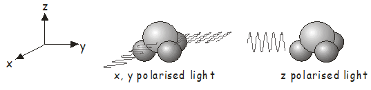
Earlier in the course, we learned how to determine the symmetry molecular orbitals. The symmetry of an electronic state is found by identifying any unpaired electrons and taking the direct product of the irreducible representations of the molecular orbitals in which they are located. The ground state of a closed-shell molecule, in which all electrons are paired, always belongs to the totally symmetric irreducible representation\(^7\). As an example, the electronic ground state of \(NH_3\), which belongs to the \(C_{3v}\) point group, has \(A_1\) symmetry. To find out which electronic states may be accessed by absorption of a photon, we need to determine the irreducible representations for the electric dipole operator \(\hat{\boldsymbol{\mu}}\). Light that is linearly polarized along the \(x\), \(y\), and \(z\) axes transforms in the same way as the functions \(x\), \(y\), and \(z\) in the character table\(^8\). From the \(C_{3v}\) character table, we see that \(x\)- and \(y\)-polarized light transforms as \(E\), while \(z\)-polarized light transforms as \(A_1\). Therefore:
- For \(x\)- or \(y\)-polarized light, \(\Gamma_\hat{\boldsymbol{\mu}} \otimes \Gamma_{\Psi 1}\) transforms as \(E \otimes A_1 = E\). This means that absorption of \(x\)- or \(y\)-polarized light by ground-state \(NH_3\) (see figure below left) will excite the molecule to a state of \(E\) symmetry.
- For \(z\)-polarized light, \(\Gamma_\hat{\boldsymbol{\mu}} \otimes \Gamma_{\Psi 1 }\) transforms as \(A_1 \otimes A_1 = A_1\). Absorption of \(z\)-polarized light by ground state \(NH_3\) (see figure below right) will excite the molecule to a state of \(A_1\) symmetry.
Of course, the photons must also have the appropriate energy, in addition to having the correct polarization to induce a transition.
We can carry out the same analysis for \(H_2O\), which belongs to the \(C_{2v}\) point group. We showed previously that \(H_2O\) has three molecular orbitals of \(A_1\) symmetry, two of \(B_1\) symmetry, and one of \(B_2\) symmetry, with the ground state having \(A_1\) symmetry. In the \(C_{2v}\) point group, \(x\)-polarized light has \(B_1\) symmetry, and can therefore be used to excite electronic states of this symmetry; \(y\)-polarized light has \(B_2\) symmetry, and may be used to access the \(B_2\) excited state; and \(z\)-polarized light has \(A_1\) symmetry, and may be used to access higher lying \(A_1\) states. Consider our previous molecular orbital diagram for \(H_2O\).
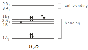
The electronic ground state has two electrons in a \(B_2\) orbital, giving a state of \(A_1\) symmetry (\(B_2 \otimes B_2 = A_1\)). The first excited electronic state has the configuration \((1B_2)^1(3A_1)^1\) and its symmetry is \(B_2 \otimes A_1 = B_2\). It may be accessed from the ground state by a \(y\)-polarized photon. The second excited state is accessed from the ground state by exciting an electron to the \(2B_1\) orbital. It has the configuration \((1B_2)^1(2B_1)^1\), its symmetry is \(B_2 \otimes B_1 = A_2\). Since neither \(x\)-, \(y\)- or \(z\)-polarized light transforms as \(A_2\), this state may not be excited from the ground state by absorption of a single photon.
Vibrational transitions in molecules
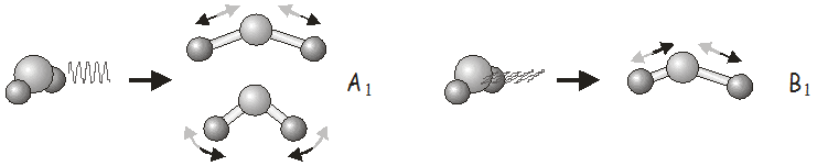
Similar considerations apply for vibrational transitions. Light polarized along the \(x\), \(y\), and \(z\) axes of the molecule may be used to excite vibrations with the same symmetry as the \(x\), \(y\) and \(z\) functions listed in the character table.
For example, in the \(C_{2v}\) point group, \(x\)-polarized light may be used to excite vibrations of \(B_1\) symmetry, \(y\)-polarized light to excite vibrations of \(B_2\) symmetry, and \(z\)-polarized light to excite vibrations of \(A_1\) symmetry. In \(H_2O\), we would use \(z\)-polarized light to excite the symmetric stretch and bending modes, and \(x\)-polarized light to excite the asymmetric stretch. Shining \(y\)-polarized light onto a molecule of \(H_2O\) would not excite any vibrational motion.
Raman Scattering
If there are vibrational modes in the molecule that may not be accessed using a single photon, it may still be possible to excite them using a two-photon process known as Raman scattering\(^9\). An energy level diagram for Raman scattering is shown below.
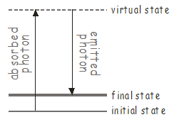
The first photon excites the molecule to some high-lying intermediate state, known as a virtual state. Virtual states are not true stationary states of the molecule (i.e. they are not eigenfunctions of the molecular Hamiltonian), but they can be thought of as stationary states of the ‘photon + molecule’ system. These types of states are extremely short lived, and will quickly emit a photon to return the system to a stable molecular state, which may be different from the original state. Since there are two photons (one absorbed and one emitted) involved in Raman scattering, which may have different polarizations, the transition dipole for a Raman transition transforms as one of the Cartesian products \(x^2\), \(y^2\), \(z^2\), \(xy\), \(xz\), \(yz\) listed in the character tables.
Vibrational modes that transform as one of the Cartesian products may be excited by a Raman transition, in much the same way as modes that transform as \(x\), \(y\), or \(z\) may be excited by a one-photon vibrational transition.
In \(H_2O\), all of the vibrational modes are accessible by ordinary one-photon vibrational transitions. However, they may also be accessed by Raman transitions. The Cartesian products transform as follows in the \(C_{2v}\) point group.
\[\begin{array}{clcl} A_1 & x^2, y^2, z^2 & B_1 & xz \\ A_2 & sy & B_2 & yz \end{array} \tag{27.5}\]
The symmetric stretch and the bending vibration of water, both of \(A_1\) symmetry, may therefore be excited by any Raman scattering process involving two photons of the same polarization (\(x\)-, \(y\)- or \(z\)-polarized). The asymmetric stretch, which has \(B_1\) symmetry, may be excited in a Raman process in which one photon is \(x\)-polarized and the other \(z\)-polarized.
\(^7\)It is important not to confuse molecular orbitals (the energy levels that individual electrons may occupy within the molecule) with electronic states (arising from the different possible arrangements of all the molecular electrons amongst the molecular orbitals, e.g. the electronic states of \(NH_3\) are NOT the same thing as the molecular orbitals we derived earlier in the course. These orbitals were an incomplete set, based only on the valence \(s\) electrons in the molecule. Inclusion of the \(p\) electrons is required for a full treatment of the electronic states. The \(H_2O\) example above should hopefully clarify this point.
\(^8\)‘\(x\)-polarized’ means that the electric vector of the light (an electromagnetic wave) oscillates along the direction of the \(x\) axis.
\(^9\)You will cover Raman scattering (also known as Raman spectroscopy) in more detail in later courses. The aim here is really just to alert you to its existence and to show how it may be used to access otherwise inaccessible vibrational modes.