Solid State Experiments

The solid state NMR community has developed hundreds of techniques to investigate different parts of the NMR Hamiltonian. This section gives a brief, by no means comprehensive of a few techniques that are helpful in probing select interactions. Additional resources useful for understanding 2D NMR are available.

Magic Angle Spinning (MAS) NMR

For a spin 1/2 nucleus, the CSA and the dipolar coupling significantly broaden the solids lineshape, even in crystalline compounds. By inspecting the Hamiltonians of each interaction, the \(3cos(\theta)-1\) term appears. If this term was set to zero the dipolar coupling would go to zero. The CSA would only be dependent on \(\phi\) and \(\eta\). Rapid rotation about this angle would average all \(\phi\) leading to a purely isotropic lineshapes. This is the logic behind (MAS) NMR. In this experiment, the sample is physically rotated around the magic angle at very high spinning speeds, on the order of kHz. The magic angle can be solved for numerically by,

\[3 \cos\theta-1=0\]

\[ \theta=54.74 = \text{Magic Angle}\]

The chemical shift can be related to the individual orientation of the crystal in the rotor to the PAS using Euler angles, \(\alpha, \beta,\gamma\). This conversion gives a chemical shift of

\[-\omega_0{\sigma_{iso}+[A_1 \cos(\omega_r t+\gamma)+B_1 \sin(\omega_r t+\gamma)]+[A_2\cos(2\omega_r t+2\gamma)+B_2\sin(\omega_r t+2\gamma]}\]

where

\[\begin{align} A_1 &=\frac{2}{3} \sqrt{2} \sin \beta cos\beta [\cos^2\alpha (\sigma_{xx}^{PAS}- \sigma_{zz}^{PAF}) +\sin^2\alpha (\sigma_{yy}^{PAS}- \sigma_{zz}^{PAF})] \\[4pt] B_1 &=\frac{2}{3} \sqrt{2} \sin \alpha \cos\alpha \sin\beta (\sigma_{xx}^{PAS} -\sigma_{zz}^{PAF}) \\[4pt] A_2 &=\frac{1}{3} ((\cos^2 \beta \cos^2\alpha -\sin^2\alpha) (\sigma_{xx}^{PAS} -\sigma_{zz}^{PAF}) +(\cos^2\beta \sin^2\alpha- \cos^2\alpha) (\sigma_{yy}^{PAS} -\sigma_{zz}^{PAF})) \\[4pt] B_2 &=-\frac{2}{3} \sin\alpha \cos\alpha \cos\beta (\sigma_{xx}^{PAS}- \sigma_{zz}^{PAF}) \end{align}\]

This expression is useful when considering incomplete averaging of the CSA by MAS. Incomplete averaging of the CSA occurs when the spinning frequency is less than the size of the CSA. The first term of this equation is the isotropic component and the remaining terms are all dependent on the spinning frequency \(\omega_r\). When the CSA averaging is incomplete, these terms describe rotation echoes observed in the FID. Rotational echoes form as the crystallite moves with the rotor. Due to the rotation, the orientation of the crystallite changes which changes the shielding around the nucleus. Once the sample returns to its original starting position, the next rotation will have the crystallite sampling the same orientation for the same time, imposing a separate FID on the FID. The additional FIDs, denoted by the red arrows, are known as rotational echoes and are denoted as sharp spike in the time dimension, shown in the figure below. Rotational echoes are easy to identify as they appear in the FID as sharp spikes spaced every \(\frac{1}{\omega_r}\). When the sample is spinning faster than the anisotropy, the shielding lags behind the spinning speed and the crystallite shielding will not experience the same set of values over the same time period prevention rotational echo formation.

Figure 9. Rotational echoes in the FID are denoted by the red arrows. After a FT the rotational echoes become equally spaced spinning sidebands at integer multiples of the spinning speed (8kHz).

Figure 10. Effect of spinning speed on the CSA ( \(\Delta=200ppm\) )of ⁷⁷Se.

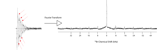
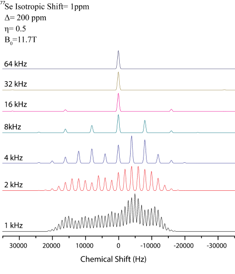
Fourier transforming this results in characteristic spinning sidebands which appear at integer multiples of the spinning speed. Spinning sideband patterns, shown above, provide information about the CSA and are therefore helpful to have when performing structural studies. In this figure, \(\delta=200ppm\) and \(\eta=0.5\).However, if a compound has multiple sites all with large CSA values, the spectrum becomes complicated and the isotropic peaks cannot be identified a priori. To identify the isotropic positions, a Herzfeld Berger analysis of the sideband patters may be performed. In a Herzfeld Berger analysis, spectra are collected at different spinning speeds. The more spinning speeds at which the spectrum is collected, the easier the assignment of the peaks. The sidebands appear at integer multiples of the rotor speed, while the isotropic peaks remain constant. Thus to find the peaks you only need to locate those peaks that do not move when the spinning speed is changed. The relative intensities of the isotropic peaks will not change, while the sideband patterns will change intensities depending on the spinning speed. However, an isotropic peak may be overlapping with a sideband, giving artificial intensity to that peak.

As alluded to earlier, the CSA parameters may be derived from the sideband patterns. When doing this one must consider a few things:

1. The dipolar coupling. If the spinning speed is not large enough to average the dipolar coupling between nuclei this can give additional sidebands which when fit lead to inaccurate determination of CSA
2. At least 4 sidebands in order to have enough degrees of freedom to accurately fit the chemical shift tensor. The chemical shift tensor is 3x3 matrix. If the matrix is diagonalized, there are 6 remaining values; 3 isotropic and 3 anisotropic. The anisotropy may be fit using 3 values in which case you need 3+1 degrees of freedom to fit accurately.

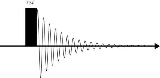
Below is a typical pulse sequence used for MAS experiments. It is sometimes called pulse and acquire, as only a \(\frac{\pi}{2}\) pulse is used and the spectrum is immediately acquired. The pulse doesn't need to be \(\frac{\pi}{2}\). In fact, normally a pulse with a smaller tip angle is used in order to acquire more scans in a shorter time. The optimum tip angle at which the signal is maximized at the shortest time is called the Ernst angle.

Figure 11. Pulse sequence for MAS experiment

Hahn Echo

The Hahn echo sequence is named after Erwin Hahn, who in the 1950's discovered that by applying a pulse with one phase and then another pulse with a different phase, the signal would refocus and form what is known as an echo. There are many different types of echoes including solids echoes, Solomon echoes, and Hahn echoes. The Hahn echo is particularly important for spin =¹/₂ nuclei. By applying a \(\frac{\pi}{2}\) pulse waiting a set delay and then pulsing with a \(\pi\) pulse results in an echo forming. The delay between the \(\frac{\pi}{2}\) and the \(\pi\) pulses will be the time at which the echo reaches its maximum value, as shown in the pulse sequence below. In this experiment the delay is an integer multiple of the rotor period, or rotor-synchronized. This synchronization is important in order to retain any information about the CSA. Obviously if the rotor is no longer rotor synchronized the CSA will refocus at a different time yielding different (fake) interactions. The Hahn echo is often used to shift the signal out in time to negate any pulse ringdown effects that may add artificial broadening to the spectrum.

Figure 12. Pulse sequence for Hahn echo experiment

To understand how an echo forms an analogy to runners on a track (shown below) is used. Initially, all of the runners (circles) are at the starting line. Each runner (different colored circle) represents one spin in the ensemble. After the race starts, the runners begin to race around the track, separating based on speed (arrows). This is equivalent to T₂ relaxation in the NMR system. However, as theses runners begin to lose their coherence a whistle is blown and the runners all turn around and run back toward the starting line at EXACTLY the same speed as before. When they reach the starting line they are all in phase again. This is the echo that is seen in the NMR experiment. Thus the Hahn echo can be used to measure T₂ processes.

Figure 13. Graphic depiction of how a Hahn echo forms. Initially, each runner (spin) is at the starting line (in phase). After some time the runners begin to separate based on their speed (spins precess at slightly different speed). At some time a whistle is blown and the runner turn and race back to the start at exactly the same speed (\(\pi\) pulse). After the same amount of time the runners come back to the starting line (echo formation).

Solids Echo

In quadrupolar nuclei, the refocusing of the spins into echoes becomes challenging as there are multiple energy levels and certain transitions are forbidden \(\Delta m \neq \pm 1\). Consequently, treating the quadrupolar nuclei with the Hahn echo sequence results in incomplete refocusing (Some of the runners do not hear the whistle and turn around). This leads to different interactions which need to be discussed more thoroughly. However, if instead a \(\frac{\pi}{2}\) pulse is used instead of the \(\pi\) pulse, the central transitions will experience the spin flip and reform a solids (quadrupolar) echo. The main advantage of this type of echo is that it includes no broadening to do satellite transitions and is therefore more quantitative than a Hahn echo for quadrupolar nuclei.

Figure 14. Solids echo pulse sequence

Multiple Quantum MAS (MQMAS)

Figure 16. MQMAS pulse sequence

MQMAS is a high resolution 2D NMR technique that allows for an isotropic spectrum of a quadrupolar nucleus to be detected. Frydman and Harwood showed that by manipulating spin coherences using pulses, the second and fourth rank Legendre Polynomials can be averaged over the entire experiment. Separating the experiment into 2 time domains t₁ and t₂ and setting the Legendre polynomials to zero yields

\[C_4(I,m_1)t_1+C_4(I, m_2)t_2=0\].

Experimentally, t₁ can be chosen and the resulting echo will form at t₂. However, m₂ is fixed as the final transition needs to be ¹/₂ so the signal can be detected. Solving for t₂ yields:

\[t_2=kt_1\]

\[k=\frac{C_4(I,m_1)}{C_4(I,\frac{1}{2})}\]

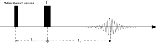
In order to complete this experiment, the MQ transition must first be excited. This can be accomplished using a very short \(\frac{\pi}{12}\) pulse. After waiting t₁, the spins are then reconverted into the central transition so they can be detected. The resultant echo consists of spins which have satisfied the averaging of the fourth rank polynomials and therefore only contain isotropic information. Next, t₁ is varied and the resultant echo is measured. The signal then evolves on a diagonal (k) which is then sheared an FT in both dimensions giving a v₁^' correlated with the isotropic and anisotropic components.

Figure 17. Processing of the raw MQMAS data. After a 2D FT and shear the isotropic and anisotropic components of the signal can be correlated. Initially the signal evolves on a diagonal proportional to k.

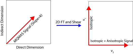
in this figure

\[\nu_1=\frac{34\nu_{iso}-60\nu_0}{9}\]

and

\[\nu_2=\nu_{iso}+3\nu_0-21\nu_4(\theta,\phi)\]

Two Dimensional Phase Adjusted Spinning Sidebands (2D PASS)

Figure 18. 2D PASS pulse sequence. The timings between the pulses are modulated to satisfy the PASS equations.

The 2D PASS experiment is an experiment which separates the CSA from the isotropic chemical shift. The pulse sequence consists of a \(\frac{\pi}{2}\) pulse followed by a train of 5 \(\pi\) pulses which are spaced at timings given by the PASS equations. The PASS equations are complex and will not be discussed further. Timings for the pulses may be found in the paper published by Antzutkin et al. in 1995.

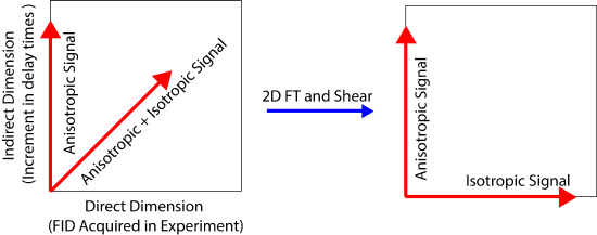
The goal of this experiment is to separate the CSA into a separate dimension from the isotropic chemical shift. The basic principle is that the CSA may be separated out by changing the timings between the pi pulses. The change in the timings allows for the isotropic part of the chemical shift to evolve as a function of the timings and the CSA is directly acquired in each 1D slice. The two are then related to one another by a shearing transformation. The data acquisition and evolution of the CSA and isotropic chemical shift are shown in the figure below.

Figure 19. Processing of the 2D data. After a 2D FT and a shearing transformation, the anisotropic and isotropic components of the CSA can be related.

Dynamic Angle Spinning (DAS)

Unlike MQMAS which manipulated the spin of the nuclei, DAS manipulates the orientation of the spins in the rotor. As can be seen in the quadrupolar equations, no one angle can allow for complete averaging the of the quadrupolar interactions. However, solving these equations individually leads to sets of angles (left as an exercise for the reader).

Several techniques have been developed in order to exploit the different angles.

Double Rotation: This technique places a smaller rotor oriented at a different orientation inside a rotor which spins at the magic angle. The rotor inside also spins, which averages 2 of the above interactions. This is an extremely challenging experiment and the inner rotor is only able to spin at a max of 3 kHz.

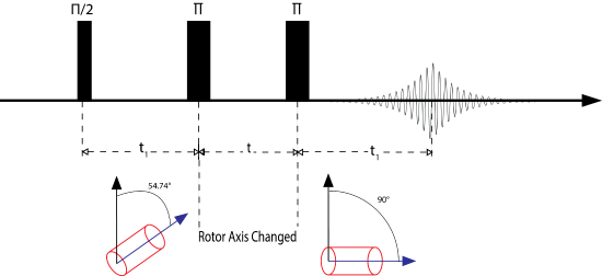
Magic Angle Flipping: In this technique, the rotor is physically reoriented by a stepper motor during the experiment. Commonly, the experiment is performed at the magic angle and then is reoriented to 90 degrees to reintroduce the anisotropy. In this way the anisotropy can be correlated to the isotropic chemical shift, much like the 2D PASS experiment. However, when using a quadrupolar nucleus, the sample can be reoriented to another "magic" angle which will average the remainder of the quadrupolar interaction. In order for a successful experiment \(\tau\), the time it takes to switch the rotor must be shorter than T1 or no signal will be observed.

Figure 20. Pulse sequence and rotor position for the DAS experiment.

References

MAS References

1. Fyfe,C. A., Massbruger, H., Yannoni, C.S. J. Mag. Res. 36 (1979) 61-68 doi:10.1016/0022-2364(79)90215-4
2. Herzfled, J., Berger, A.E., J. Chem Phys. 73 (1980) 6021-6030 doi:10.1063/1.440136

MQMAS References

1. Goldbourt, A., Madhu, P., Chemical Monthly. 133 (2002) 1497-1534. doi:10.1007/s00706-002-0502-y
2. Medek, A., Frydman, L., J. Braz. Chem Soc. 10 (1999) 263-277. doi:10.1021/ja00156a015
3. Frydman, L., Harwood , J.S., J. Am.Chem. SOc. 117 (1995) 5367 ISSN:0103-5053

2D PASS References

1. Dixon, W.T., J. Chem. Phys. 77 (1982) 1800-1809
2. Antzutkin, O. N., Shekar, S.C., Levitt, M. H., J. Magnetic Rsonance A. 115 (1995) 7-19 doi:10.1006/jmra.1995.1142
3. Kaseman, D. C., Hung, I., Gan, Z., Sen, S. J. Phys. Chem. B. 117 (2013)949-954 doi:10.1021/jp311320t
4. Kaseman, D. C. Endo, T. Sen, S. J. Non-Cryst. Solids. 359 (2013) 33-39 doi:10.1016/j.jnoncrysol.2012.09.030
5. Hung, I., Edwards, T, Sen, S., Gan, Z., J. Mag Res. 221 (2012) 103-109 doi:10.1016/j.jmr.2012.05.013
6. Fayon, F., Bessada, C., Douy, A. Massiot, D. J. Mag. Res. 137 (1999) 116-121 doi:10.1006/jmre.1998.1641
7. Davis, M. C., Shookman, K. M., Sillaman, J. D., Grandinetti, P. J., J Mag Res. 210 (2011) 51-58 doi:10.1016/j.jmr.2011.02.008

Echo References

1. Anderson, A. G., Garwin, R. L., Hahn, E.L., Horton, J.W., Tucker, G.L., Walker, R.M., J. Appl. Phys. 26 (1955) 1324-1338 doi:10.1063/1.1721903
2. Hahn, E. L., Phys. Rev. 80 (1950) 580-594 doi:10.1103/PhysRev.80.580 doi:10.1103/PhysRev.93.639
3. Hahn, E. L., Herzog, B., Phys. Rev. 93 (1954) 639-640 doi 10.1103/PhysRev.93.639
4. Hahn, E. L., Maxwell, D. E., Phys Rev. 84 (1951) 1246-1247 doi:10.1103/PhysRev.84.1246
5. Hahn, E. L., Maxwell, D. E., Phys Rev 88 (1952) 1070-1084 doi:10.1103/PhysRev.88.1070
6. Rowan, L. G., Hahn, E. L., Mims, W. B., Phys Rev. 137 (1965) A61 doi:10.1103/PhysRev.137.A61

CPMG References

1. Carr, H. Y., Purcell, E. M., Phys Rev. 94 (1954) 630-638 doi:10.1103/PhysRev.94.630
2. Meiboom, S., Gill, D., Review of Scientific Instruments. 29 (1958) 688-691 doi:10.1063/1.1716296
3. Hung, I., Edwards, T, Sen, S., Gan, Z., J. Mag Res. 221 (2012) 103-109 doi:10.1016/j.jmr.2012.05.013
4. Baltisberger, J. H., Waler, B. J., Keeler, E. G., Kaseman, D. C., Sanders, K. J., Grandinetti, P. J., J Chem Phys. 136 (2012) doi:10.1063/1.4728105

DAS References

1. Chmelka, B.F., Mueller, K. T., Pines, A., Stebbins, J., Wu, Y., Zwanziger, J. W., Nature. 339 (1989) 42-43 doi:10.1038/339042a0
2. Eastman, M. A., Grandinetti, P.J., Lee, Y. K., Pines, A., J. Mag. Res. 98 (1990) 333-341 doi:10.1016/0022-2364(92)90136-u
3. Farnan, I., Grandinetti, P. J., Baltisberger, J. H., Stebbines, J. H., Werner, U., Eastman, M.A., Pines, A., Nature. 358 (1992) 31-35 doi:10.1038/358031a0
4. Mueller, K. T., Baltisberger, J. H., Wooten, E. W., Pines, A., J. Phys Chem. 96 (1992) 7001-7004 doi:10.1021/j100196a028
5. Mueller, K. T., Chingas, G.C., Pines, A., Review Scientific Instruments. 62 (1991) 1445-1452 doi:10.1063/1.1142465
6. Meuller, K. T., Sun, B.Q., Chingas, G. C., Zwanziger, J. W., Terao, T., Pines, A. J Mag. Res. 86 (1990) 470-487 doi:10.1016/0022-2364(90)90025-5
7. Meuller, K.T., Wooten, E.W., Pines, A., J. Mag. Res, 92 (1991) 620-627 doi:10.1016/0022-2364(91)90359-2