4.27: The Michelson Interferometer and Fourier Transform Spectroscopy

A Michelson interferometer with a movable mirror in one arm is an essential element in Fourier Transform (FT) spectroscopy.

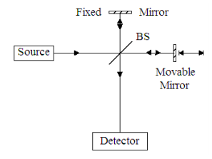
A source illuminates a 50‐50 beam splitter (BS). After the beam splitter the photons are in a linear superposition of being both transmitted and reflected. By convention a 90^o phase shift is assigned to the reflected beam.

\[ | S \rangle \rightarrow \frac{1}{ \sqrt{2}} \left[ |T \rangle + i | R \rangle \right] \nonumber \]

Mirrors return the reflected and transmitted photons to the beam splitter where they evolve into the following superpositions.

\[ | R \rangle \rightarrow \frac{1}{ \sqrt{2}} \left[ |D \rangle + i | S \rangle \right] \nonumber \]

\[ | T \rangle \rightarrow \frac{ \text{exp} \left( i \frac{2 \pi \delta}{ \lambda} \right)}{ \sqrt{2}} \left[ S \rangle + i|D \rangle \right] \nonumber \]

The reflected beam is in a superposition of being transmitted to the detector and reflected back to the source, while the transmitted beam is in a superposition of being transmitted to the source and reflected to the detector. The exponential term in equation (3) is the phase shift acquired by the transmitted beam due to any path difference between the two arms created by the movable mirror.

The history of the source photons is obtained by substitution of equations (2) and (3) into equation (1).

\[ |S \rangle \rightarrow \frac{1}{2} \left[ \left( \text{exp} \left( i \frac{2 \pi \delta}{ \lambda} \right) - 1 \right) |S \rangle + i \left( \text{exp} \left( i \frac{2 \pi \delta}{ \lambda} \right) +1 \right) |D \rangle \right] \nonumber \]

The intensity of the radiation arriving at the detector (D) is the absolute magnitude squared of its coefficient in equation(4).

\[ I_D ( \delta) = \left| i \left( \text{exp} \left( i \frac{2 \pi \delta}{ \lambda} \right) + 1 \right) \right|^2 = \frac{1}{2} \left[ \cos \frac{2 \pi \delta}{ \lambda} +1 \right] \nonumber \]

Thus for a single‐frequency source the intensity at the detector as a function of δ traces a cosine function.

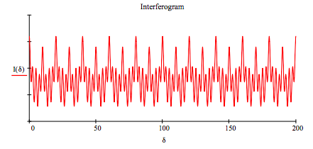
In FT‐IR spectroscopy the source is a ʺglowerʺ that emits a broad range of infrared frequencies. In this case the signal at the detector is the sum of of intensities of the individual photons. This is called an interferogram and has the following mathematical form.

\[ I ( \delta) = \sum_j \left| i \left( \text{exp} \left( i \frac{2 \pi \delta}{ \lambda_j} \right) +1 \right) \right|^2 = \sum_j \frac{1}{2} \left[ \cos \left( \frac{2 \pi \delta}{ \lambda_j} \right) + 1 \right] \nonumber \]

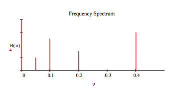
The interferogram is obtained by measuring the intensity at the detector as a function of the path difference (δ) also called the retardation. In the next step the intensity of the frequencies present in the source beam are recovered by the following Fourier Transform.

\[ B( \nu) = \int I ( \delta) \text{exp} (i 2 \pi \delta \nu) d \delta \nonumber \]

To illustrate the FT method we will assume that the source beam only contains four wavelengths or frequencies.

\[ \begin{matrix} \text{Wavelength:} & \lambda_1 = 20 & \lambda_2 = 10 & \lambda_3 = 5 & \lambda_4 = 2.5 \\ \text{Intensities:} & B_1 = 2 & B_2 = 5 & B_3 = 3 & B_4 = 6 & \text{Frequencies:} & \frac{1}{ \lambda_1} = 0.05 & \frac{1}{ \lambda_2} = 0.1 & \frac{1}{ \lambda_3} = 0.2 & \frac{1}{ \lambda_4} = 0.4 \end{matrix} \nonumber \]

Generate interferogram:

\[ \begin{matrix} I ( \delta) = & \frac{1}{2} \left( \cos \left( 2 \pi \frac{ \delta}{ \lambda_1} \right) +1 \right) B_1 + \frac{1}{2} \left( \cos \left( 2\pi \frac{ \delta}{ \lambda_2} \right) + 1 \right) B_2 ... \\ & + \frac{1}{2} \left( \cos \left( 2 \pi \frac{ \delta}{ \lambda_3} \right) +1 \right) B_3 + \frac{1}{2} \left( \cos \left( 2 \pi \frac{ \delta}{ \lambda_4} \right) +1 \right) B_4 \end{matrix} \nonumber \]

Display interferogram:

\[ \delta = 0, .1 ... 200 \nonumber \]

Fourier transform interferogram to recover frequencies and intensities:

\[ \begin{matrix} B( \nu) = \int_{0}^{200} I ( \delta) \text{exp}(i 2 \pi \delta \nu) d \delta & \nu = 0, 0.005 .. .5 \end{matrix} \nonumber \]

This calculation reveals how a Michelson interferometer is used to measure the wavelengths or frequencies present in the source beam. In a FT‐IR instrument the source ideally contains all the IR frequencies. The sample is placed between the beam splitter and the detector and an absorption spectrum is measured.