
4.26: HD-Like NMR Spectrum Calculated Using Tensor Algebra
- Page ID
- 151315

In section 7.12.3 of Atoms and Molecules, Karplus and Porter consider the nuclear magnetic resonance of HD. In this tutorial it is treated as analogous to the traditional AB system, except that HD consists of a spin 1/2 nucleus interacting with a spin 1 nucleus. Using arbitrary values for the chemical shifts and coupling constant, a tensor algebra calculation yields a model nmr spectrum. Related tutorials on the AB and ABC systems are also available in this tutorial section.
\[ \begin{matrix} \text{Chemical shifts:} & \nu_H = 400 & \nu_D = 200 & \text{Coupling constant:} & J_{HD} = 30 \end{matrix} \nonumber \]
Nuclear spin and identity operators for the proton (the proton is a spin 1/2 particle):
\[ \begin{matrix} IH_x = \frac{1}{2} \begin{pmatrix} 0 & 1 \\ 1 & 0 \end{pmatrix} & IH_y = \frac{1}{2} \begin{pmatrix} 0 & -i \\ i & 0 \end{pmatrix} & IH_z = \frac{1}{2} \begin{pmatrix} 1 & 0 \\ 0 & -1 \end{pmatrix} & IH = \begin{pmatrix} 1 & 0 \\ 0 & 1 \end{pmatrix} \end{matrix} \nonumber \]
Nuclear spin and identity operators for the deuteron (the deuteron is a spin 1 particle):
\[ \begin{matrix} ID_x = \frac{1}{ \sqrt{2}} \begin{pmatrix} 0 & 1 & 0 \\ 1 & 0 & 1 \\ 0 & 1 & 0 \end{pmatrix} & ID_y = \frac{1}{ \sqrt{2}} \begin{pmatrix} 0 & -i & 0 \\ i & 0 & -i \\ 0 & i & 0 \end{pmatrix} & ID_z = \begin{pmatrix} 1 & 0 & 0 \\ 0 & 0 & 0 \\ 0 & 0 & -1 \end{pmatrix} & ID = \begin{pmatrix} 1 & 0 & 0 \\ 0 & 1 & 0 \\ 0 & 0 & 1 \end{pmatrix} \end{matrix} \nonumber \]
Hamiltonian representing the interaction of nuclear spins with the external magnetic field in tensor format:
\[ \widehat{h}_{MagField} = - \nu_H \hat{I}_z^H - \nu_D \hat{I}_z^H = - \nu_H \hat{I}_z^H \otimes \hat{I}_D - \nu_D \hat{I}_H \otimes \hat{I}_z^D \nonumber \]
Implementing the operator using Mathcadʹs command for the tensor product, kronecker, is as follows.
\[ H_{MagField} = - \nu_H \text{kronecker} \left( IH_z,~ID \right) - \nu_D \text{kronecker} \left(IH,~ID_z \right) \nonumber \]
Hamiltonian representing the interaction of nuclear spins with each other in tensor format:
\[ \hat{H}_{SpinSpin} = J_{HD} \left( \hat{I}_x^H \otimes \hat{I}_x^D + \hat{I}_y^H \otimes \hat{I}_y^D + \hat{I}_z^H \otimes \hat{I}_z^D \right) \nonumber \]
Implementation of the operator in the Mathcad programming environment:
\[ H_{SpinSpin} = J_{HD} \left( \text{kronecker} \left( IH_x,~ID_x \right) + \text{kronecker} \left( IH_y,~ID_y \right) + \text{kronecker} \left( IH_z,~ID_z \right) \right) \nonumber \]
The total Hamiltonian spin operator is now calculated and displayed.
\[ H = H_{MagField} + H_{SpinSpin} \nonumber \]
\[ H = \begin{pmatrix} -385 & 0 & 0 & 0 & 0 & 0 \\ 0 & -200 & 0 & 21.213 & 0 & 0 \\ 0 & 0 & -15 & 0 & 21.213 & 0 \\ 0 & 21.213 & 0 & -15 & 0 & 0 \\ 0 & 0 & 21.213 & 0 & 200 & 0 \\ 0 & 0 & 0 & 0 & 0 & 415 \end{pmatrix} \nonumber \]
Calculate and display the energy eigenvalues and associated eigenvectors of the Hamiltonian.
\[ \begin{matrix} i = 1 .. 6 & E = \text{sort(eigenvals(H))} & C^{<i>} = \text{eigenvec} \left( H,~E_i \right) \end{matrix} \nonumber \]
\[ \text{augment} \left( E,~C^T \right)^T = \begin{pmatrix} -385 & -202.401 & -17.073 & -12.599 & 202.073 & 415 \\ 1 & 0 & 0 & 0 & 0 & 0 \\ 0 & 0.994 & 0 & 0.112 & 0 & 0 \\ 0 & 0 & 0.995 & 0 & 0.097 & 0 \\ 0 & -0.112 & 0 & 0.994 & 0 & 0 \\ 0 & 0 & -0.097 & 0 & 0.995 & 0 \\ 0 & 0 & 0 & 0 & 0 & 1 \end{pmatrix} \nonumber \]
The HD composite nuclear spin states expressed in tensor format are as follows:
\[ \begin{matrix} | \frac{1}{2},~ 1 \rangle = \begin{pmatrix} 1 \\ 0 \end{pmatrix} \otimes \begin{pmatrix} 1 \\ 0 \\ 0 \end{pmatrix} = \begin{pmatrix} 1 \\ 0 \\ 0 \\ 0 \\ 0 \\ 0 \end{pmatrix} & | \frac{1}{2},~ 0 \rangle = \begin{pmatrix} 1 \\ 0 \end{pmatrix} \otimes \begin{pmatrix} 0 \\ 1 \\ 0 \end{pmatrix} = \begin{pmatrix} 0 \\ 1 \\ 0 \\ 0 \\ 0 \\ 0 \end{pmatrix} & | \frac{1}{2},~ -1 \rangle = \begin{pmatrix} 1 \\ 0 \end{pmatrix} \otimes \begin{pmatrix} 0 \\ 0 \\ 1 \end{pmatrix} = \begin{pmatrix} 0 \\ 0 \\ 1 \\ 0 \\ 0 \\ 0 \end{pmatrix} \\ | - \frac{1}{2},~ 1 \rangle = \begin{pmatrix} 0 \\ 1 \end{pmatrix} \otimes \begin{pmatrix} 1 \\ 0 \\ 0 \end{pmatrix} = \begin{pmatrix} 0 \\ 0 \\ 0 \\ 1 \\ 0 \\ 0 \end{pmatrix} & | - \frac{1}{2},~ 0 \rangle = \begin{pmatrix} 0 \\ 1 \end{pmatrix} \otimes \begin{pmatrix} 0 \\ 1 \\ 0 \end{pmatrix} = \begin{pmatrix} 0 \\ 0 \\ 0 \\ 0 \\ 1 \\ 0 \end{pmatrix} & | - \frac{1}{2},~ -1 \rangle = \begin{pmatrix} 0 \\ 1 \end{pmatrix} \otimes \begin{pmatrix} 0 \\ 0 \\ 1 \end{pmatrix} = \begin{pmatrix} 0 \\ 0 \\ 0 \\ 0 \\ 0 \\ 1 \end{pmatrix} \end{matrix} \nonumber \]
The nmr selection rule is that only one nuclear spin can flip during a transition and that ΔI = +/‐ 1. Therefore, the transition probability matrix given the above nuclear spin assignments for the HD system is:
\[ T = \begin{pmatrix} 0 & 1 & 0 & 1 & 0 & 0 \\ 1 & 0 & 1 & 0 & 1 & 0 \\ 0 & 1 & 0 & 0 & 0 & 1 \\ 1 & 0 & 0 & 0 & 1 & 0 \\ 0 & 1 & 0 & 1 & 0 & 1 \\ 0 & 0 & 1 & 0 & 1 & 0 \end{pmatrix} \nonumber \]
Calculate the transition intensities and frequencies.
\[ \begin{matrix} i = 1 .. 6 & j = 1 .. 6 & I_{i,~j} = \left[ C^{<i>T} \left( TC^{<j>} \right) \right] & V_{i,~j} = \left| E_i - E_j \right| \end{matrix} \nonumber \]
Display the calculated HD nmr spectrum:
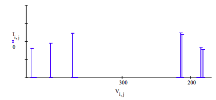
As expected, we see that the single proton resonance on the left is split into three transitions due to the three deuteron spin orientations, and that the two deuteron resonances are each split into two transitions due to the two proton spin orientations.
The frequencies of all possible transitions are presented in the following matrix.
\[ V = \begin{pmatrix} 0 & 182.599 & 367.927 & 372.401 & 587.073 & 800 \\ 182.599 & 0 & 185.328 & 189.803 & 404.474 & 617.401 \\ 367.927 & 185.328 & 0 & 4.474 & 219.146 & 432.073 \\ 372.401 & 189.803 & 4.474 & 0 & 214.672 & 427.599 \\ 587.073 & 404.474 & 219.146 & 214.672 & 0 & 212.927 \\ 800 & 617.401 & 432.073 & 427.599 & 212.927 & 0 \end{pmatrix} \nonumber \]
Some of these transitions are forbidden by the selection rule as can be seen in the following intensity matrix.
\[ I = \begin{pmatrix} 0 & 0.776 & 0 & 1.224 & 0 & 0 \\ 0.776 & 0 & 0.816 & 0 & 0.948 & 0 \\ 0 & 0.816 & 0 & 1.903 \times 10^{-5} & 0 & 0.806 \\ 1.224 & 0 & 1.903 \times 10^{-5} & 0 & 1.236 & 0 \\ 0 & 0.948 & 0 & 1.236 & 0 & 1.194 \\ 0 & 0 & 0.806 & 0 & 1.194 & 0 \end{pmatrix} \nonumber \]
On the basis of the frequency and intensity tables we make the following assignments for the various allowed transition for the proton and deuteron.
\[ \begin{matrix} \left| \frac{1}{2},~-1 \right\rangle \xrightarrow{432.1} \left| \frac{-1}{2},~ -1 \right\rangle & \left| \frac{1}{2},~ 0 \right\rangle \xrightarrow{404.5} \left| \frac{-1}{2},~0 \right\rangle & \left| \frac{1}{2},~1 \right\rangle \xrightarrow{372.4} \left| \frac{-1}{2},~1 \right\rangle \\ \left| \frac{-1}{2},~1 \right\rangle \xrightarrow{214.7} \left| \frac{-1}{2},~ 0 \right\rangle & \left| \frac{1}{2},~ 0 \right\rangle \xrightarrow{212.9} \left| \frac{-1}{2},~-1 \right\rangle & \left| \frac{1}{2},~0 \right\rangle \xrightarrow{185.3} \left| \frac{1}{2},~-1 \right\rangle & \left| \frac{1}{2},~1 \right\rangle \xrightarrow{182.6} \left| \frac{-1}{2},~0 \right\rangle \end{matrix} \nonumber \]