4.8: Visualizing the Formally Forbidden Overtone Vibrational Transitions in HCl

Using the harmonic oscillator model, the selection rule for molcecular vibrations is ∆v = +/- 1. However, overtone transitions (∆v = 2, 3, ..) are observed experimentally. In what follows it will be shown that under the Morse oscillator (anharmonic) model, overtone vibrational transitions are weakly allowed.

Schroedinger's equation for the Morse oscillator model for \(\ce{HCl}}\) is integrated numerically for the first five energy states. (Integration algorithm taken from J. C. Hansen, J. Chem. Educ. Software, 8C2, 1996.)

Set integration parameters (in atomic units):

\[ \begin{matrix} n = 150& xmin = 1.4 & xmax = 8 & \Delta = \frac{xmax - xmin}{n-1} \end{matrix} \nonumber \]

Enter the Morse parameters for HCl (in atomic units):

\[ \begin{matrix} \mu = 1785.64 & D = .1655 & \beta = 1.0051 & x_e = 2.4086 \end{matrix} \nonumber \]

Calculate position vector, the potential energy matrix, and the kinetic energy matrix. Then combine them into a total energy matrix.

\[ \begin{matrix} i = 1 .. n & j = 1 .. n & x_i = xmin + (i-1) \Delta \end{matrix} \nonumber \]

\[ \begin{matrix} V_{i,~j} = \text{if} \left[ i = j,~D \left[ 1 - exp \left[ - \beta (x_i - x_e ) \right] \right]^2,~0 \right] & T_{i,~j} = \text{if} \left[ i=j,~ \frac{ \pi^2}{6 \mu \Delta^2},~ \frac{(-1)^{i-j}}{(i-j)^2 \mu \Delta} \right] \end{matrix} \nonumber \]

Hamiltonian matrix: H = T + V

Calculate eigenvalues: E = sort(eigenvals(H))

Display selected eigenvalues: m = 1 .. 6

\[ E_m = \begin{array}{|c|} \hline 0.00677149 \\ \hline 0.01989016 \\ \hline 0.03244307 \\ \hline 0.04443024 \\ \hline 0.05585166 \\ \hline \end{array} \nonumber \]

Calculate selected eigenvectors: Ψ(k) = eigenvec(H, E_k)

Plot diagonal elements of potential energy matrix and selected eigenfunctions: Vpot_i = V_{i, i}

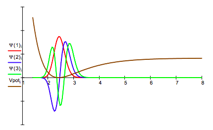
Because of the way the integration algorithm is implemented the initial index is m = 1. This corresponds to the v = 0 vibrational ground state. In other words, subtract 1 from the m index to get the v quantum number.*

Demonstrate numerically that the solutions form an orthonormal set:

\[ \begin{matrix} \sum_i ( \Psi (1)_i )^2 = 1.00 & \sum_i ( \Psi (2)_i )^2 = 1.00 & \sum_i ( \Psi (3)_i )^2 = 1.00 \\ \sum_i ( \Psi (1)_i \Psi (2)_i ) = 0.00 & \sum_i ( \Psi (1)_i \Psi (3)_i ) = 0.00 & \sum_i ( \Psi (2)_i \Psi (3)_i ) = 0.00 \end{matrix} \nonumber \]

Calculate the transition dipole moment to demonstrate that the v = 0 to v = 2 transition, which is forbidden for the harmonic oscillator, is (slightly) allowed. Compare this result to v = 0 to v = 1, v = 1 to v=2 transitions which are allowed. (See * above.)

\[ \begin{matrix} \sum_i ( \Psi (1)_i x_i \Psi (3)_i ) = -0.01 & \sum_i ( \Psi (1)_i x_i \Psi (2)_i ) = 0.14 & \sum_i ( \Psi (2)_i x_i \Psi (3)_i ) = 0.21 \end{matrix} \nonumber \]

Animate these transitions to confirm that they lead to oscillating dipole character.

Select quantum numbers of initial and final states:

\[ \begin{matrix} v_i = 1 & v_f = 3 \end{matrix} \nonumber \]

Energy of transition:

\[ \begin{matrix} \Delta E = E_{vf} - E_{vi} & \Delta E = 0.02567158 \end{matrix} \nonumber \]

Define animation parameter:

\[ t = \frac{ \text{FRAME}}{10^{-8}} \nonumber \]

Time-dependent superposition of initial and final states:

\[ \Phi_i = \frac{ \Psi (vi)_i exp (-i E_{vi} t) + \Psi (vf)_i exp(-i E_{vf} t)}{ \sqrt{2}} \nonumber \]

To animate click on Tools, Animation, Record and follow the instructions in the dialog box. Recommended setting: From 0 To 40 in 5 Frames/Sec.