4.7: A Rudimentary Analysis of the Vibrational-Rotational HCl Spectrum

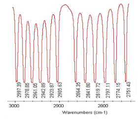
This analysis assumes an harmonic‐oscillator, non‐rigid rotor model for the vibrational and rotational degrees of freedom of gas‐phase HCl. In other words, the magnitude of the rotational constant depends on the vibrational state of the molecule. Using the portion of the H³⁵Cl vibrational‐rotational spectrum provided below, this model will be used to calculate the following molecular parameters: ν₀, B₀, B₁, B_e, α_e, r₀, r₁, r_e, and k.

A simple algebraic method, rather than a sophisticated statistical analysis, will be used to extract HClʹs molecular parameters from the spectroscopic data. We will see that although the model and the method of analysis are rudimentary, the results compare rather well with literature values for the molecular parameters. This exercise might serve as an introduction to a more rigorous and thorough statistical analysis. The equations for the R‐branch and P‐branch transitions appropriate for this model are given below.

\[ \begin{matrix} \nu_R(J) = \textcolor{red}{ \nu_0} B_1 (J+1)(J+2) - B_0 J(J+1) & \nu_p (J) = \textcolor{red}{ \nu_0} + B_1 (J-1)J-B_0 J(J+1) \end{matrix} \nonumber \]

where

\[ \begin{matrix} B_{ \nu} = \frac{h}{8 \pi^2 c \mu r_{ \nu}^2} & B_{ \nu} = B_e - \alpha_e \left( \nu + \frac{1}{2} \right) \end{matrix} \nonumber \]

Fundamental constants, conversion factors and atomic masses:

\[ \begin{matrix} h = 6.6260755 (10)^{-34} \text{joule sec} & c = 2.99792458 (10)^8 \frac{m}{sec} & u = 1.66054 10^{-27} kg & pm = 10^{-12} m \\ m_H = 1.0078 u & m_{Cl} = 34.9688 u \end{matrix} \nonumber \]

Calculate the reduced mass of HCl:

\[ \begin{matrix} \mu = \frac{m_H + m_{Cl}}{m_H + m_{Cl}} & \mu = 1.627 \times 10^{-27} kg \end{matrix} \nonumber \]

Obtain several P- and R-branch transitions from the spectrum:

\[ \begin{pmatrix} \text{Transition} & P(2) & P(1) & R(0) & R(1) \\ \frac{ \text{Frequency}}{cm^{-1}} & 2841.80 & 2864.35 & 2905.63 & 2923.87 \end{pmatrix} \nonumber \]

Set up and solve a system of equations to calculate ν₀, B₀ and B₁ by selecting data from the table above.

\[ \begin{array}{c|c} \begin{pmatrix} \nu_0 & B_0 & B_1 \end{pmatrix} = \begin{pmatrix} \nu_p (2) = 2841.80 cm^{-1} \\ \nu_p (1) = 2864.35 cm^{-1} \\ \nu_R (0) = 2905.63 cm^{-1} \end{pmatrix} & _{float,~5}^{solve,~ \begin{pmatrix} \nu_0 \\ B_0 \\ B_1 \end{pmatrix}} \rightarrow \begin{pmatrix} \frac{2885.6}{cm} \\ \frac{10.638}{cm} \\ \frac{10.002}{cm} \end{pmatrix} \end{array} \nonumber \]

Use the values of B₀ and B₁ to calculate B_e and α_e:

\[ \begin{array}{c|c} \begin{pmatrix} B_e & \alpha_e \end{pmatrix} = \begin{pmatrix} B_0 = B_e - \alpha_e \frac{1}{2} \\ B_1 = B_e - \alpha_e \frac{3}{2} \\ \nu_R (0) = 2905.63 cm^{-1} \end{pmatrix} & _{float,~5}^{solve,~ \begin{pmatrix} B_e \\ \alpha_e \end{pmatrix}} \rightarrow \begin{pmatrix} \frac{10.956}{cm} \\ \frac{.63600}{cm} \end{pmatrix} \end{array} \nonumber \]

Now calcuate r₀, r₁, and r_e using the values of B₀, B₁ and B_e.

\[ \begin{matrix} r_0 = \sqrt{ \frac{h}{8 \pi^2 c \mu B_0}} & r_0 = 127.189 pm & r_1 = \sqrt{ \frac{h}{8 \pi^2 c \mu B_1}} & r_1 = 131.171 pm \\ r_e = \sqrt{ \frac{h}{8 \pi^2 c \mu B_e}} & r_e = 125.33 pm \end{matrix} \nonumber \]

Calculate the force constant using the value of ν₀.

\[ \begin{matrix} \begin{array}{c|c} k = \nu_0 = \frac{1}{2 \pi c} \sqrt{ \frac{k}{ \mu}} & _{float,~4}^{solve,~k} \rightarrow .4806e-1 \frac{m^2}{sec^2 cm^2} kg \end{array} & k = 480.6 \frac{newton}{m} \end{matrix} \nonumber \]

Compare the calculated parameter values with the literature values.

\[ \begin{pmatrix} \frac{ \text{Molecular}}{ \text{Parameter}} & \frac{ \text{Calcuated}}{ \text{Value}} & \frac{ \text{Literature}}{ \text{Value}} & \% \text{Error} \\ \frac{ \nu_0}{cm^{-1}} & 2885.6 & 2886 & 0.014 \\ \frac{B_0}{cm^{-1}} & 10.638 & 10.440 & 1.90 \\ \frac{B_1}{cm^{-1}} & 10.002 & 10.136 & 1.32 \\ \frac{B_e}{cm^{-1}} & 10.956 & 10.593 & 3.43 \\ \frac{ \alpha_e}{ cm_{-1}} & 0.6360 & 0.307 & 107 \\ \frac{r_0}{pm} & 127.2 & 128.3 & 0.86 \\ \frac{r_1}{pm} & 131.2 & 130.2 & 0.77 \\ \frac{r_e}{pm} & 125.3 & 127.4 & 1.65 \\ \frac{k}{newton~m^{-1}} & 480.6 & 516.3 & 6.92 \end{pmatrix} \nonumber \]

Summary: Given the simplicity of the model (harmonic‐oscillator, non‐rigid rotor) and the rudimentary algebraic (as opposed to rigorous statistical) method of analysis, the results are quite respectable. Naturally, results will vary depending on the P‐ and R‐branch transitions used to calculate the molecular parameters.