4.2: A Particle-in-a-Box Model for Color Centers

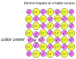
Electrons trapped (see figure below) in anion vacancies of alkali halide salts absorb visible radiation and cause the typically white solids to appear colored.* A simple explanation of this phenomenon is that due to the wave nature of matter (the basic postulate of quantum theory), the energy of a trapped particle, such as an electron, is quantized. This permits a simple interpretation of the absorption spectra (and, therefore, the color) of F‐centers. It is assumed that a photon of visible light promotes the trapped electron from its ground state to its first excited state.

This simplest model for the electron under these conditions is to assume that it behaves like a particle in a cubic box. The allowed energy levels of an electron in a cubic box are,

\[ E = \frac{h^2}{8 ma^2} \left[ \left( n_x \right)^2 + \left( n_y \right)^2 + \left( n_z \right)^2 \right] \nonumber \]

where, h is Planckʹs constant, m is the electron mass, a is the box dimension, and n_x, n_y, and n_z are quantum numbers.

On the basis of this simple model the first allowed transition is given by

\[ \Delta E = \frac{hc}{ \lambda} = E_f - E_i = \frac{h^2}{8ma^2} \left[ \left(2^2 + 1^2 + 1^2 \right) - \left( 1^2 + 1^2 + 1^2 \right) \right] \nonumber \]

where c is the speed of light and λ is the wavelength of the photon of light absorbed. This expression can be re‐written as follows:

\[ \begin{matrix} \lambda = \frac{8mc}{3h} a^2 = 1099 a^2 & \text{(where } λ \text{ and a are given in nanometers)} \end{matrix} \nonumber \]

As equation (3) shows, the model predicts that the wavelength maximum is directly proportional to the box dimension squared.

Reasonable agreement between experimental absorbance maxima and the model can be obtained by assuming that the electron is restricted to a cube the size of one unit cell. This is shown below by doing a linear regression analysis on equation (3) assuming that the exponent of a is an adjustable parameter. In other words, it is assumed that the wavelength maximum is directly proportional to aⁿ, where a is the lattice constant and n is the parameter to be determinded.

The data below are the lattice constant and wavelength maximum for the following alkali halides: LiF, NaF, LiCl, KF, NaCl, NaBr, KCl, NaI, RbCl, KBr, RbBr, KI, and RbI.

i = 1 .. 13

\[ \begin{matrix} a_i = & \lambda_i = \\ \begin{array}{|c|} \hline .402 \\ \hline .462 \\ \hline .514 \\ \hline .534 \\ \hline .562 \\ \hline .596 \\ \hline .628 \\ \hline .646 \\ \hline .654 \\ \hline .658 \\ \hline .686 \\ \hline .706 \\ \hline .732 \\ \hline \end{array} & \begin{array}{|c|} \hline 250 \\ \hline 341 \\ \hline 385 \\ \hline 455 \\ \hline 458 \\ \hline 540 \\ \hline 556 \\ \hline 588 \\ \hline 609 \\ \hline 625 \\ \hline 694 \\ \hline 689 \\ \hline 756 \\ \hline \end{array} \end{matrix} \nonumber \]

Equation (3) is transformed into a linear function by taking the logarithm of both sides of the equation. This yields: ln(λ) = n ln(a) + ln(1099). This is, of course, the familiar: y = slope*x + intercept.

\[ \begin{matrix} y_i = \ln( \lambda_i ) & x_i = \ln (a_i) \\ \text{a = slope(x, y)} & \text{b = slope(x, y)} & \text{c = corr(x, y)} \\ \text{Slope:} & a = 1.7943 & \text{Intercept:} & b = 7.1841 \\ \text{Correlation coefficient:} & c = 9.9499 \times 10^{-1} \end{matrix} \nonumber \]

The data and the fit to the data are displayed below. The fit is good and the optimum value of n is reasonably close to the theoretical value of 2. Ways to increase the sophistication of the model are discussed below.

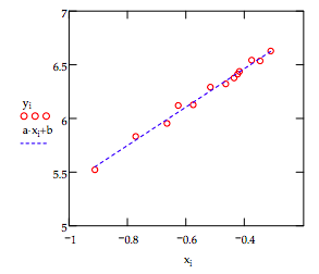
It is clear from the figure above that the simple model employed here accounts for the trend in the data. More sophisticated models would assume that the electron occupied a finite potential well. In other words that some tunneling into the potential barrier would be permitted. In addition to cubic wells, it would not be difficult to perform an analysis assuming that the trapped electrons occupy finite spherical potential wells.

*The F‐center (electron trapped in an anion vacancy) can be formed by the ionization of the halide anion as follows: X‐ + hν ‐‐‐‐‐‐‐> X + e‐. The neutral X drifts away and the negatively charged electron takes its place as the anion in the crystal structure.

Reference: G. P. Hughes, ʺColor Centers: An example of a particle trapped in a finite potential wellʺ, American Journal of Physics 45, 948, (1977).