8.92: Quantum Key Distribution Using a Mach-Zehnder Interferometer

Charles H. Bennett proposed the following Mach-Zehnder interferometer for quantum key distribution (Physical Review Letters 68, 3121 (1992)).

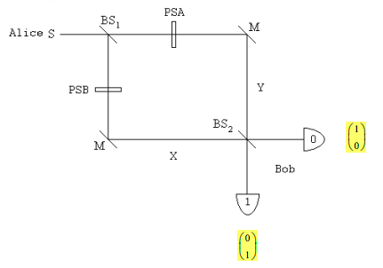
Alice's source at the left supplies single-photon states, which are split by a symmetric beam splitter BS₁ into a superposition being present in both arms of a Mach-Zehnder interferometer (MZI). Alice (PSA) applies a random 0-, 90-, 180-, or 270-degree phase shift in one arm and Bob (PSB) applies a random 0- or 90-degree phase shift in the other arm. Mirrors direct the photon to a second beam splitter creating two photon paths to each detector and thereby allowing for interference between the paths. After photon detection by Bob, Alice and Bob agree publicly to keep only those results for which their phase shifts differ by 0 or 180 degrees, settings for which the photons behave deterministically at the second beam splitter.

Direction of propagation vectors:

\[ \begin{matrix} x = \begin{pmatrix} 1 \\ 0 \end{pmatrix} & y = \begin{pmatrix} 0 \\ 1 \end{pmatrix} \end{matrix} \nonumber \]

Matrix operators for the interferometer components:

\[ \begin{matrix} \text{Beam splitter:} & \text{BS:} = \frac{1}{ \sqrt{2}} \begin{pmatrix} 1 & i \\ i & 1 \end{pmatrix} & \text{Mirror:} & \text{M:} = \begin{pmatrix} 0 & 1 \\ 1 & 0 \end{pmatrix} & \text{Phase shift:} \begin{pmatrix} e&{i~PSA} & 0 \\ 0 & e&{i~PSB} \end{pmatrix} \end{matrix} \nonumber \]

Construct a Mach-Zehnder interferometer using these components.

\[ \text{MZI(PSA, PSB) = BS M} \begin{pmatrix} e^{i~PSA} & 0 \\ 0 & e^{i~PSB} \end{pmatrix} \text{BS} \nonumber \]

\[ \begin{matrix} \text{Probability Detector 0 will fire:} & \text{Probability Detector 1 will fire:} \\ \text{Detector_0(PSA, PSB) =} \left( \left| x^T \text{MZI(PSA, PSB) x} \right| \right) ^2 & \text{Detector_1(PSA, PSB) =} \left( \left| y^T \text{MZI(PSA, PSB) x} \right| \right)^2 \end{matrix} \nonumber \]

For each of eight possible phase shift settings calculate the probability that detectors |0> and |1> will register the arrival of a photon.

The PSA/PSB settings for which a photon behaves deterministically are highlighted.

\[ \begin{matrix} ~ & ~ & \text{Detector} = \begin{pmatrix} 1 \\ 0 \end{pmatrix} = 0 & \text{Detector} = \begin{pmatrix} 0 \\ 1 \end{pmatrix} = 1 \\ \textcolor{magenta}{PSA = 0 deg} & \textcolor{magenta}{PSB = 0 deg} & \textcolor{magenta}{Detector_0(PSA, PSB) = 1} & \textcolor{magenta}{Detector_1(PSA, PSB) = 0} \\ \text{PSA = 0 deg} & \text{PSB= 90 deg} & \text{Detector_0(PSA, PSB) = 0.5} & \text{Detector_1(PSA, PSB) = 0.5} \\ \text{PSA = 90 deg} & \text{PSB= 0 deg} & \text{Detector_0(PSA, PSB) = 0.5} & \text{Detector_1(PSA, PSB) = 0.5} \\ \textcolor{magenta}{PSA = 90 deg} & \textcolor{magenta}{PSB = 90 deg} & \textcolor{magenta}{Detector_0(PSA, PSB) = 1} & \textcolor{magenta}{Detector_1(PSA, PSB) = 0} \\ \textcolor{magenta}{PSA = 180 deg} & \textcolor{magenta}{PSB = 0 deg} & \textcolor{magenta}{Detector_0(PSA, PSB) = 0} & \textcolor{magenta}{Detector_1(PSA, PSB) = 1} \\ \text{PSA = 180 deg} & \text{PSB= 270 deg} & \text{Detector_0(PSA, PSB) = 0.5} & \text{Detector_1(PSA, PSB) = 0.5} \\ \text{PSA = 270 deg} & \text{PSB= 0 deg} & \text{Detector_0(PSA, PSB) = 0.5} & \text{Detector_1(PSA, PSB) = 0.5} \\ \textcolor{magenta}{PSA = 270 deg} & \textcolor{magenta}{PSB = 90 deg} & \textcolor{magenta}{Detector_0(PSA, PSB) = 0} & \textcolor{magenta}{Detector_1(PSA, PSB) = 1} \end{matrix} \nonumber \]

Demonstrate that the detection results at each detector are completely random. In other words, that if someone was monitoring Bob's detectors he or she would see no pattern in the results.

The settings of phase shifters PSA and PSB are changed randomly by Alice and Bob. So given a large number of runs, each pair of settings shown above will occur with probability 1/8 or 12.5%. Overall each detector will register a photon in half the runs.

\[ \begin{matrix} \textcolor{magenta}{Detector = \begin{pmatrix} 1 \\ 0 \end{pmatrix}} & \frac{1 + \frac{1}{2} + \frac{1}{2} + 1 + 0 + \frac{1}{2} + \frac{1}{2} + 0}{8} \rightarrow \frac{1}{2} & \textcolor{magenta}{Detector = \begin{pmatrix} 0 \\ 1 \end{pmatrix}} & \frac{0 + \frac{1}{2} + \frac{1}{2} + 0 + 1 + \frac{1}{2} + \frac{1}{2} + 1}{8} \rightarrow \frac{1}{2} \end{matrix} \nonumber \]

Demonstrate the use of a secret key to exchange a secure message between a sender and a receiver.

Coding and Decoding a Message

\[ \begin{matrix} j = 1 .. 25 & \text{Key}_j = \text{trunc(rnd(2))} & \text{Key}^T = \begin{pmatrix} 0 & 0 & 1 & 0 & 1 & 0 & 1 & 0 & 0 & 0 & 1 & 0 & 0 & 1 & 1 & 0 & 0 & 0 & 1 & 1 & 1 & 1 & 1 & 0 & 1 \end{pmatrix} \\ ~ & \text{Mes}_j = \text{trunc(rnd(2))} & \textcolor{magenta}{ \text{Mes}^T = \begin{pmatrix} 1 & 1 & 1 & 0 & 1 & 0 & 1 & 0 & 0 & 1 & 1 & 0 & 1 & 0 & 1 & 1 & 1 & 1 & 0 & 0 & 1 & 1 & 0 & 0 & 1 \end{pmatrix}} \\ \text{CMes}_j = \text{Mes}_j \oplus \text{Key}_j & \text{CMes}^T = \begin{pmatrix} 1& 1 & 0 & 0 & 0 & 0 & 0 & 0 & 0 & 1 & 0 & 0 & 1 & 1 & 0 & 1 & 1 & 1 & 1 & 1 & 0 & 0 & 1 & 0 & 0 \end{pmatrix} \\ \text{DMes}_j = \text{CMes}_j \oplus \text{Key}_j & \textcolor{magenta}{ \text{Mes}^T = \begin{pmatrix} 1 & 1 & 1 & 0 & 1 & 0 & 1 & 0 & 0 & 1 & 1 & 0 & 1 & 0 & 1 & 1 & 1 & 1 & 0 & 0 & 1 & 1 & 0 & 0 & 1 \end{pmatrix}} \end{matrix} \nonumber \]

It is clear by inspection that the message has been accurately decoded. This is confirmed by calculating the difference between the message and the decoded message.

\[ \text{(DMes} - \text{Mes)}^T = \begin{pmatrix} 0 & 0 & 0 & 0 & 0 & 0 & 0 & 0 & 0 & 0 & 0 & 0 & 0 & 0 & 0 & 0 & 0 & 0 & 0 & 0 & 0 & 0 & 0 & 0 & 0 \end{pmatrix} \nonumber \]

In 2000 Anton Zeilinger and his research team sent an encrypted photo of the fertility goddess Venus of Willendorf from Alice to Bob, two computers in two buildings about 400 meters apart. The figure summarizing this achievement first appeared in Physical Review Letters and later in a review article in Nature.

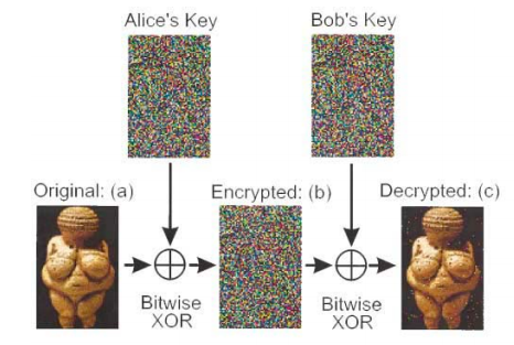
By extending the previous example to two dimensions, it easy to produce a rudimentary simulation of the experiment. Bitwise XOR is nothing more than addition modulo 2. (XOR = CNOT)

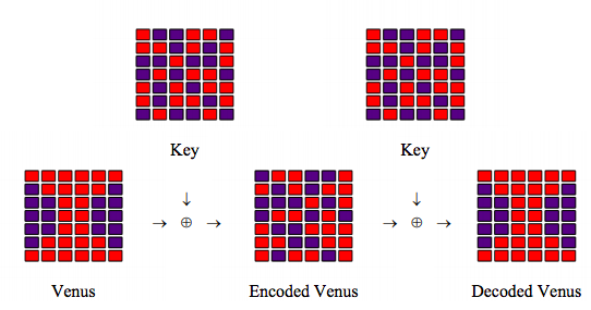
The original Venus and the shared key are represented by the following matrices, where the matrix elements are pixels that are either off (0) or on (1).

\[ \begin{matrix} \text{Venus} = \begin{pmatrix} 1 & 1 & 1 & 1 & 1 & 1 \\ 0 & 1 & 1 & 1 & 1 & 0 \\ 0 & 0 & 1 & 1 & 0 & 0 \\ 0 & 0 & 1 & 1 & 0 & 0 \\ 0 & 0 & 1 & 1 & 0 & 0 \\ 0 & 1 & 1 & 1 & 1 & 0 \\ 1 & 1 & 1 & 1 & 1 & 1 \end{pmatrix} & \text{Key} = \begin{pmatrix} 1 & 0 & 0 & 1 & 1 & 0 \\ 1 & 1 & 0 & 1 & 0 & 1 \\ 0 & 0 & 1 & 0 & 0 & 1 \\ 0 & 1 & 0 & 1 & 1 & 0 \\ 1 & 0 & 1 & 0 & 1 & 1 \\ 1 & 0 & 1 & 1 & 0 & 1 \\ 0 & 1 & 0 & 0 & 1 & 0 \end{pmatrix} \end{matrix} \nonumber \]

A coded version of Venus is prepared by adding Venus and the Key modulo 2 and sent to Bob.

\[ \begin{matrix} i = 1 .. 7 & j = 1 .. 6 & \text{CVenus}_{i,~j} = \text{Venus}_{i,~j} \oplus \text{Key}_{i,~j} & \text{CVenus} = \begin{pmatrix} 0 & 1 & 1 & 0 & 0 & 1 \\ 1 & 0 & 1 & 0 & 1 & 1 \\ 0 & 0 & 0 & 1 & 0 & 1 \\ 0 & 1 & 1 & 0 & 1 & 0 \\ 1 & 0 & 0 & 1 & 1 & 1 \\ 1 & 1 & 0 & 0 & 1& 1 \\ 1 & 0 & 1 & 1 & 0 & 1 \end{pmatrix} \end{matrix} \nonumber \]

Bob adds the key to CVenus modulo 2 and sends the result to his printer.

\[ \begin{matrix} \text{DVenus}_{i,~j} = \text{CVenus}_{i,~j} \oplus \text{Key}_{i,~j} & \text{DVenus} = \begin{pmatrix} 1 & 1 & 1 & 1 & 1 & 1 \\ 0 & 1 & 1 & 1 & 1 & 0 \\ 0 & 0 & 1 & 1 & 0 & 0 \\ 0 & 0 & 1 & 1 & 0 & 0 \\ 0 & 0 & 1 & 1 & 0 & 0 \\ 0 & 1 & 1 & 1 & 1 & 0 \\ 1 & 1 & 1 & 1 & 1 & 1 \end{pmatrix} \end{matrix} \nonumber \]

A graphic summary of the simulation:

Random key production can be implemented as follows:

\[ \begin{matrix} j = 1 .. 20 & \text{PSA}_j = \text{trunc(rnd(4)) 90 deg} & \text{PSB}_j = \text{trunc(rnd(2)) 90 deg} \end{matrix} \nonumber \]

\[ \begin{matrix} \text{Det0}_j = \left[ \left| x^T \text{BS M} \begin{pmatrix} e^{i ~PSA_j} & 0 \\ 0 & e^{i~PSB_j} \end{pmatrix} \text{BS x} \right| \right]^2 & \text{Det1}_j = \left[ \left| y^T \text{BS M} \begin{pmatrix} e^{i ~PSA_j} & 0 \\ 0 & e^{i~PSB_j} \end{pmatrix} \text{BS x} \right| \right]^2 \end{matrix} \nonumber \]

\[ \begin{matrix} \frac{PSA_j}{deg} = & \frac{PSB_j}{deg} = & \text{Det0}_j = & \text{Det1}_j = \\ \begin{array}{|c|} \hline \\ 0 \\ \hline \\ 0 \\ \hline \\ 180 \\ \hline \\ 90 \\ \hline \\ 270 \\ \hline \\ 0 \\ \hline \\ 270 \\ \hline \\ 0 \\ \hline \\ 270 \\ \hline \\ 0 \\ \hline \\ 180 \\ \hline \\ 90 \\ \hline \\ 180 \\ \hline \\ 180 \\ \hline \\ 0 \\ \hline \\ \cdots \\ \hline \end{array} & \begin{array}{|c|} \hline \\ 0 \\ \hline \\ 90 \\ \hline \\ 0 \\ \hline \\ 90 \\ \hline \\ 90 \\ \hline \\ 0 \\ \hline \\ 90 \\ \hline \\ 90 \\ \hline \\ 0 \\ \hline \\ 90 \\ \hline \\ 90 \\ \hline \\ 90 \\ \hline \\ 90 \\ \hline \\ 90 \\ \hline \\ 0 \\ \hline \\ \cdots \\ \hline \end{array} & \begin{array}{|c|} \hline \\ 1 \\ \hline \\ 0.5 \\ \hline \\ 0 \\ \hline \\ 1 \\ \hline \\ 0 \\ \hline \\ 1 \\ \hline \\ 0 \\ \hline \\ 0.5 \\ \hline \\ 0.5 \\ \hline \\ 0.5 \\ \hline \\ 0.5 \\ \hline \\ 1 \\ \hline \\ 0.5 \\ \hline \\ 0.5 \\ \hline \\ 1 \\ \hline \\ \cdots \\ \hline \end{array} & \begin{array}{|c|} \hline \\ 0 \\ \hline \\ 0.5 \\ \hline \\ 1 \\ \hline \\ 0 \\ \hline \\ 1 \\ \hline \\ 0 \\ \hline \\ 1 \\ \hline \\ 0.5 \\ \hline \\ 0.5 \\ \hline \\ 0.5 \\ \hline \\ 0.5 \\ \hline \\ 0 \\ \hline \\ 0.5 \\ \hline \\ 0.5 \\ \hline \\ 0 \\ \hline \\ \cdots \\ \hline \end{array} \end{matrix} \nonumber \]