8.89: Matrix Mechanics Analysis of the BB84 Key Distribution

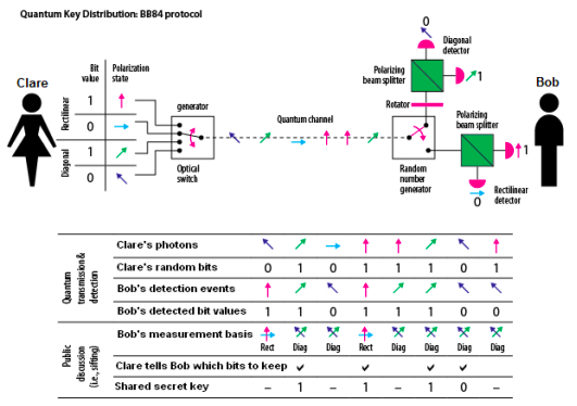
The figure below (www.nsa.gov/research/tnw/tnw201/article6.shtml) illustrates an implementation of the BB84 public key distribution protocol. Clare randomly sends Bob single photons in either the rectilinear or diagonal basis. Bob randomly chooses to measure the photons he receives in either the rectilinear or diagonal basis. The table below the figure displays typical results and how Clare and Bob use them to create a secret key.

While the key distribution protocol is clear enough from the graphic alone, the purpose of this tutorial is to show the details of its operation using the methods of matrix mechanics.

Direction of motion and polarization states are represented by the following vectors. The x-direction is horizontal in the figure above.

\[ \begin{matrix} \text{Direction of propagation states:} x = \begin{pmatrix} 1 \\ 0 \end{pmatrix} & y = \begin{pmatrix} 0 \\ 1 \end{pmatrix} \\ \text{Photon polarization states:} & v = \begin{pmatrix} 1 \\ 0 \end{pmatrix} & h = \begin{pmatrix} 0 \\ 1 \end{pmatrix} & d = \frac{1}{ \sqrt{2}} \begin{pmatrix} 1 \\ 1 \end{pmatrix} & s = \frac{1}{ \sqrt{2}} \begin{pmatrix} 1 \\ -1 \end{pmatrix} \end{matrix} \nonumber \]

There are eight propagation-polarization states which are created by tensor multiplication of the appropriate vectors.

\[ \begin{matrix} xv = \begin{pmatrix} 1 \\ 0 \end{pmatrix} \begin{pmatrix} 1 \\ 0 \end{pmatrix} & xv = \begin{pmatrix} 1 \\ 0 \\ 0 \\ 0 \end{pmatrix} & xh = \begin{pmatrix} 1 \\ 0 \end{pmatrix} \begin{pmatrix} 0 \\ 1 \end{pmatrix} & xh = \begin{pmatrix} 0 \\ 1 \\ 0 \\ 0 \end{pmatrix} & yv = \begin{pmatrix} 0 \\ 1 \end{pmatrix} \begin{pmatrix} 1 \\ 0 \end{pmatrix} & yv = \begin{pmatrix} 0 \\ 0 \\ 1 \\ 0 \end{pmatrix} & yh = \begin{pmatrix} 0 \\ 1 \end{pmatrix} \begin{pmatrix} 0 \\ 1 \end{pmatrix} & yh = \begin{pmatrix} 0 \\ 0 \\ 0 \\ 1 \end{pmatrix} \end{matrix} \nonumber \]

\[ \begin{matrix} xd = \begin{pmatrix} 1 \\ 0 \end{pmatrix} \frac{1}{ \sqrt{2}} \begin{pmatrix} 1 \\ 1 \end{pmatrix} & xd = \frac{1}{ \sqrt{2}} \begin{pmatrix} 1 \\ 1 \\ 0 \\ 0 \end{pmatrix} & xs = \begin{pmatrix} 1 \\ 0 \end{pmatrix} \frac{1}{ \sqrt{2}} \begin{pmatrix} 1 \\ -1 \end{pmatrix} & xs = \frac{1}{ \sqrt{2}} \begin{pmatrix} 1 \\ -1 \\ 0 \\ 0 \end{pmatrix} \\ yd = \begin{pmatrix} 0 \\ 1 \end{pmatrix} \frac{1}{ \sqrt{2}} \begin{pmatrix} 1 \\ 1 \end{pmatrix} & yd = \frac{1}{ \sqrt{2}} \begin{pmatrix} 0 \\ 0 \\ 1 \\ 1 \end{pmatrix} & ys = \begin{pmatrix} 0 \\ 1 \end{pmatrix} \frac{1}{ \sqrt{2}} \begin{pmatrix} 1 \\ -1 \end{pmatrix} & ys = \frac{1}{ \sqrt{2}} \begin{pmatrix} 0 \\ 0 \\ 1 \\ -1 \end{pmatrix} \end{matrix} \nonumber \]

The operators required for the BB84 implementation shown above are matrices representing the identity, mirror, rotator and polarization beam splitter, PBS.

\[ \begin{matrix} \text{I} = \begin{pmatrix} 1 & 0 \\ 0 & 1 \end{pmatrix} & \text{M} = \begin{pmatrix} 0 & 1 \\ 1 & 0 \end{pmatrix} & \text{Rotator} = \frac{1}{ \sqrt{2}} \begin{pmatrix} 1 & -1 \\ 1 & 1 \end{pmatrix} & \text{PBS} = \begin{pmatrix} 1 & 0 & 0 & 0 \\ 0 & 0 & 0 & 1 \\ 0 & 0 & 1 & 0 \\ 0 & 1 & 0 & 0 \end{pmatrix} \end{matrix} \nonumber \]

The rotator, which prepares photons for measurement in the diagonal basis, rotates the photon polarization state clockwise by 45 degrees.

\[ \begin{matrix} \text{Rotator v} = \begin{pmatrix} 0.707 \\ 0.707 \end{pmatrix} = |d \rangle & \text{Rotator h} = \begin{pmatrix} -0.707 \\ 0.707 \end{pmatrix} = - |s \rangle & \text{Rotator d} = \begin{pmatrix} 0 \\ 1 \end{pmatrix} = |h \rangle & \text{Rotator s} = \begin{pmatrix} 1 \\ 0 \end{pmatrix} = |v \rangle \end{matrix} \nonumber \]

The PBS transmits vertical and reflects horizontal photons. For example,

\[ \begin{matrix} \text{PBS xv} = \begin{pmatrix} 1 \\ 0 \\ 0 \\ 0 \end{pmatrix} = |xv \rangle & \text{PBS xh} = \begin{pmatrix} 0 \\ 0 \\ 0 \\ 1 \end{pmatrix} = yh \rangle & \text{PBS yv} = \begin{pmatrix} 0 \\ 0 \\ 1 \\ 0 \end{pmatrix} = |yv \rangle & \text{PBS yh} = \begin{pmatrix} 0 \\ 1 \\ 0 \\ 0 \end{pmatrix} = |xh \rangle \end{matrix} \nonumber \]

Interpreting Measurement Results

Suppose Bob measures Clare's photons (|v>, |h>, |d> and |s>) in the rectilinear basis. Note that the rectilinear detector is in the same direction as the photons are propagating. For |v> and |h> he correctly measures the polarization of Clare's photons. However, |d> and |s> are not eigenstates of the PBS, but superpositions of |v> and |h>, so for these photons half the time Bob will observe |v> and half the time |h>. According to quantum principles he always observes one of the eigenstates of the measurement operator. When Clare and Bob publicly discuss the result she will tell him for which events he chose the correct measurement basis.

\[ \begin{matrix} \text{PBS xv} = \begin{pmatrix} 1 \\ 0 \\ 0 \\ 0 \end{pmatrix} = xv & \text{PBS xh} = \begin{pmatrix} 0 \\ 0 \\ 0 \\ 1 \end{pmatrix} = yh & \text{PBS xd} = \begin{pmatrix} 0.707 \\ 0 \\ 0 \\ 0.707 \end{pmatrix} & \frac{1}{ \sqrt{2}} \text{(xv + yh)} = \begin{pmatrix} 0.707 \\ 0 \\ 0 \\ 0.707 \end{pmatrix} \\ ~ & ~ & \text{PBS xs} = \begin{pmatrix} 0.707 \\ 0 \\ 0 \\ -0.707 \end{pmatrix} & \frac{1}{ \sqrt{2}} \text{(xv - yh)} = \begin{pmatrix} 0.707 \\ 0 \\ 0 \\ -0.707 \end{pmatrix} \end{matrix} \nonumber \]

Suppose Bob measures Clare's photons in the diagonal basis. The diagonal detector is reached in the vertical direction via a mirror. The rotator causes a basis change so that the |d> and |s> photons become eigenvectors of the PBS. Thus for |d> or |s> Bob always gets the correct result because they have been transformed to |h> or |v>. The states |v> and |h> are transformed by the rotator into superpositions of |v> and |h>, indicating that half the time he will observe |d> and half the time |s>. When Clare and Bob publicly discuss the result she will tell him which events he chose the correct measurement basis.

\[ \begin{matrix} \text{PBS kronecker(M, Rotator) xd} = \begin{pmatrix} 0 \\ 1 \\ 0 \\ 0 \end{pmatrix} = xh & \text{PBS kronecker(M, Rotator) xs} = \begin{pmatrix} 0 \\ 0 \\ 1 \\ 0 \end{pmatrix} = yv \\ \text{PBS kronecker(M, Rotator) xv} = \begin{pmatrix} 0 \\ 0.707 \\ 0.707 \\ 0 \end{pmatrix} & \frac{1}{ \sqrt{2}} \text{(xh + yv)} = \begin{pmatrix} 0 \\ 0.707 \\ 0.707 \\ 0 \end{pmatrix} & \text{PBS kronecker(M, Rotator) xh} = \begin{pmatrix} 0 \\ 0.707 \\ -0.707 \\ 0 \end{pmatrix} & \frac{1}{ \sqrt{2}} \text{(xh - yv)} = \begin{pmatrix} 0 \\ 0.707 \\ -0.707 \\ 0 \end{pmatrix} \end{matrix} \nonumber \]

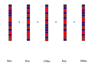
The following demonstrates how a binary message is coded and subsequently decoded using a binary key and modulo 2 arithmetic.

\[ \begin{matrix} \text{Message} & \text{Key} & \text{Coded Message} & \text{Decoded Message} \\ \text{Mes} = \begin{pmatrix} 0 \\ 1 \\ 0 \\ 0 \\ 0 \\ 1 \\ 1 \\ 0 \\ 0 \\ 1 \\ 0 \\ 1 \\ 0 \\ 1 \\ 1 \end{pmatrix} & \text{Key} = \begin{pmatrix} 0 \\ 0 \\ 1 \\ 0 \\ 1 \\ 0 \\ 1 \\ 1 \\ 0 \\ 1 \\ 0 \\ 1 \\ 1 \\ 1 \\ 0 \end{pmatrix} & \text{CMes = mod(Mes + Key, 2)} = \begin{pmatrix} 0 \\ 1 \\ 1 \\ 0 \\ 1 \\ 1 \\ 0 \\ 1 \\ 0 \\ 0 \\ 0 \\ 0 \\ 1 \\ 0 \\ 1 \end{pmatrix} & \text{DMes = mod(CMes + Key, 2)} = \begin{pmatrix} 0 \\ 1 \\ 0 \\ 0 \\ 0 \\ 1 \\ 1 \\ 0 \\ 0 \\ 1 \\ 0 \\ 1 \\ 0 \\ 1 \\ 1 \end{pmatrix} \end{matrix} \nonumber \]

It is clear by inspection that the message has been accurately decoded. This is confirmed by calculating the difference between the message and the decoded message.

\[ \text{(Mes} - \text{DMes)}^T = \begin{pmatrix} 0 & 0 & 0 & 0 & 0 & 0 & 0 & 0 & 0 & 0 & 0 & 0 & 0 & 0 & 0 \end{pmatrix} \nonumber \]

Here's a graphical representation of the coding and decoding mechanism.