8.85: Simulating the Deutsch-Jozsa Algorithm with a Double-Slit Apparatus
- Page ID
- 149125

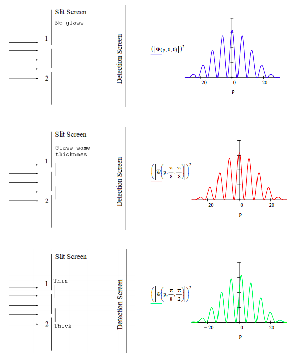
The Deutsch‐Jozsa algorithm determines if either [1] 2N numbers are either all 0 or all 1 (a constant function), or [2] half are 0 and half are 1 (a balanced function) in one step instead of up to 2N‐1 + 1 steps. For N = 1, the Deutsch‐Jozsa algorithm can be visualized as putting two pieces of glass, which may be thin (0) or thick (1), behind the apertures of a double‐slit apparatus and measuring the interference pattern of a light source illuminating the slits. If the pattern is unchanged compared to the empty apparatus, the glass pieces have the same thickness (constant function); otherwise they have different thickness (balanced function). Peter Pfeifer, ʺQuantum Computation,ʺ Access Science, Vol. 17, p. 678, slightly modified by F. R.
This is demonstrated by calculating the diffraction pattern without glass present, and with glass present of the same thickness and different thickness. The diffraction pattern is the momentum distribution, which is the Fourier transform of the slit geometry.
\[ \begin{matrix} \text{Slit positions:} & x_L = 1 & x_R = 2 & \text{Slit width:} & \delta = 2 \end{matrix} \nonumber \]
The momentum wave function with possible phase shifts θ and φ at the two slits is represented by the following superposition. The phase shifts are directly proportional to the thickness of the glass.
\[ \Psi (p, \theta, \varphi) = \frac{ \int_{x_L - \frac{ \delta}{2}}^{ x_L + \frac{ \delta}{2}} \frac{1}{ \sqrt{2 \pi}} \text{exp(-i p x)} \frac{1}{ \sqrt{ \delta}} \text{dx exp}(i \theta) + \int_{x_R -\frac{ \delta}{2}}^{x_R + \frac{ \delta}{2}} \frac{1}{ \sqrt{2 \pi}} \text{exp(-i p x)} \frac{1}{ \sqrt{ \delta}} \text{dx exp}(i \varphi)}{ \sqrt{2}} \nonumber \]
The diffraction patterns (momentum distributions) for the empty apparatus (θ = φ = 0), for an apparatus with glass pieces of the same thickness (θ = φ = π/8) and for one that has glass of different thickness (θ = π/8 ϕ = π/2) behind the slits are displayed below.
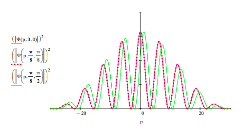
Another look at the calculations with graphical support on the left is provided below.