
8.83: Factoring Using Shor's Quantum Algorithm
- Page ID
- 149123

This tutorial presents a toy calculation dealing with quantum factorization using Shor's algorithm. Before beginning that task, traditional classical factorization is reviewed with the example of finding the prime factors of 15. As shown below the key is to find the period of ax modulo 15, where a is chosen randomly.
\[ \begin{matrix} a = 4 & N = 5 & & f(x) = mod \left( a^x,~N \right) & Q = 8 & x = 0 .. Q - 1\end{matrix} \nonumber \]
\[ \begin{matrix} x = \begin{array}{|c|} \hline \\ 0 \\ \hline \\ 1 \\ \hline \\ 2 \\ \hline \\ 3 \\ \hline \\ 4 \\ \hline \\ 5 \\ \hline \\ 6 \\ \hline \\ 7 \\ \hline \end{array} & f(x) = \begin{array}{|c|} \hline \\ 1 \\ \hline \\ 4 \\ \hline \\ 1 \\ \hline \\ 4 \\ \hline \\ 1 \\ \hline \\ 4 \\ \hline \\ 1 \\ \hline \\ 4 \\ \hline \end{array} \end{matrix} \nonumber \]
Seeing that the period of f(x) is two, the next step is to use the Euclidian algorithm by calculating the greatest common denominator of two functions involving the period and a, and the number to be factored, N.
\[ \begin{matrix} \text{period = 2} & \text{ged} \left( a^{ \frac{ \text{period}}{2}} - 1,~N \right) = 3 & \text{ged} \left( a^{ \frac{ \text{period}}{2}} + 1,~N \right) = 3 \end{matrix} \nonumber \]
Factoring 15 by this method is trivial because it is the product of two small prime numbers. However, if N is the product of two large primes this method is impractical because finding the periodicity of f(x) would not be possible by inspection as it is above. If f(x) were plotted it would appear to be random noise with no recognizable periodic structure. Shor recognized that the discrete Fourier transform (or, quantum Fourier transform) provided an efficient method for finding the period of f(x) when N is the product of two extremely large prime numbers. So the contribution that quantum mechanics may eventually make to code breaking is efficiently finding the periodicity of f(x).
We proceed by ignoring the fact that we already know that the period of f(x) is 2 and demonstrate how it is determined using a quantum (discrete) Fourier transform. After the registers are loaded with x and f(x) using a quantum computer, they exist in the following superposition.
\[ \frac{1}{ \sqrt{Q}} \sum_{x=0}^{Q-1} |x \rangle | f(x) \rangle = \frac{1}{2} \left[ |0 \rangle |1 \rangle + |1 \rangle |4 \rangle + |2 \rangle |1 \rangle + |3 \rangle |4 \rangle + \cdots \right] = \frac{1}{2} \left[ \left( |0 \rangle + |2 \rangle \right) |1 \rangle + \left( |1 \rangle + |3 \rangle \right) |4 \rangle + \cdots \right] \nonumber \]
The rearrangement on the right collects terms on the f(x) values. Now the x values appear in pairs with their f(x) partners. Note that the period of 2 is discernable in each pair of x values. After (|0 > + |2 >) the next pair is offset by 1. The Fourier transform on the x-register removes the offset, clearly revealing the period of 2.
In preparation for the Fourier transform the superposition is written as a sum of vector tensor products.
\[ \begin{matrix} \frac{1}{2} \left[ \begin{pmatrix} 1 \\ 0 \\ 0 \\ 0 \end{pmatrix} \begin{pmatrix} 0 \\ 1 \\ 0 \\ 0 \end{pmatrix} + \begin{pmatrix} 0 \\ 1 \\ 0 \\ 0 \end{pmatrix} \begin{pmatrix} 0 \\ 0 \\ 0 \\ 1 \end{pmatrix} + \begin{pmatrix} 0 \\ 0 \\ 1 \\ 0 \end{pmatrix} \begin{pmatrix} 0 \\ 1 \\ 0 \\ 0 \\ 0 \end{pmatrix} + \begin{pmatrix} 0 \\ 0 \\ 0 \\ 1 \end{pmatrix} \begin{pmatrix} 0 \\ 0 \\ 0 \\ 0 \\ 1 \end{pmatrix} \right] = \frac{1}{2} \left[ \begin{pmatrix} 1 \\ 0 \\ 1 \\ 0 \end{pmatrix} \begin{pmatrix} 0 \\ 1 \\ 0 \\ 0 \\ 0 \end{pmatrix} + \begin{pmatrix} 0 \\ 1 \\ 0 \\ 1 \end{pmatrix} \begin{pmatrix} 0 \\ 0 \\ 0 \\ 0 \\ 1 \end{pmatrix} \right] \\ \frac{1}{2} \begin{pmatrix} 0 & 1 & 0 & 0 & 0 & 0 & 0 & 0 & 0 & 1 & 0 & 1 & 0 & 0 & 0 & 0 & 0 & 0 & 0 & 1 \end{pmatrix}^T \end{matrix} \nonumber \]
The next step is to find the period of f(x) by performing a quantum Fourier transform (QFT) on the input register, |x>. The identity operation (do nothing) acts on the second register.
\[ \begin{matrix} Q = 4 & m = 0 .. Q - 1 & n = 0 .. Q - 1 & QFT_{m,~n} = \frac{1}{ \sqrt{Q}} \text{exp} \left( i \frac{2 \pi m n}{Q} \right) & I = \text{identity(5)} \end{matrix} \nonumber \]
The result of the QFT is:
\[ \begin{matrix} \text{kronecker(QFT, I)} \frac{1}{2} \begin{pmatrix} 0 \\ 1 \\ 0 \\ 0 \\ 0 \\ 0 \\ 0 \\ 0 \\ 0 \\ 1 \\ 0 \\ 1 \\ 0 \\ 0 \\ 0 \\ 0 \\ 0 \\ 0 \\ 0 \\ 1 \end{pmatrix} = \begin{pmatrix} 0 \\ 0.5 \\ 0 \\ 0 \\ 0.5 \\ 0 \\ 0 \\ 0 \\ 0 \\ 0 \\ 0 \\ 0.5 \\ 0 \\ 0 \\ -0.5 \\ 0 \\ 0 \\ 0 \\ 0 \\ 0 \end{pmatrix} & \text{expressed in tensor format} & \frac{1}{2} \begin{pmatrix} 0 \\ 1 \\ 0 \\ 0 \\ 1 \\ 0 \\ 0 \\ 0 \\ 0 \\ 0 \\ 0 \\ 1 \\ 0 \\ 0 \\ -1 \\ 0 \\ 0 \\ 0 \\ 0 \\ 0 \end{pmatrix} = \frac{1}{2} \left[ \begin{pmatrix} 1 \\ 0 \\ 0 \\ 0 \end{pmatrix} \begin{pmatrix} 0 \\ 1 \\ 0 \\ 0 \\ 1 \end{pmatrix} + \begin{pmatrix} 0 \\ 0 \\ 1 \\ 0 \end{pmatrix} \begin{pmatrix} 0 \\ 1 \\ 0 \\ 0 \\ -1 \end{pmatrix} \right] \end{matrix} \nonumber \]
The calculation at this point is summarized as follows:
\[ QFT \frac{1}{ \sqrt{2}} \sum_{x=0}^{Q-1} |x \rangle |f(x) \rangle = \frac{1}{2} \left[ |0 \rangle \left( |1 \rangle ||4 \rangle \right) + |2 \rangle \left( |1 \rangle - |4 \rangle \right) \right] \nonumber \]
Recalling that x-register originally was a superposition involving 0, 1, 2, and 3, we see that the QFT brought about constructive and destructive interference because now the x-register (blue) contains only 0 and 2. This gives us a period of 2 and we can now proceed to the classical calculation that was demonstrated earlier. The details of how the QFTon the x-register gives rise to interference is given in the summary below.
Recommended reading: Two insightful analyses of quantum mechanics' role in factoring by David Mermin appear in the April and October 2007 issues of Physics Today. The first is titled "What has quantum mechanics to do with factoring?" and the second "Some curious facts about quantum factoring." Chapter 5 in Julian Brown's The Quest for the Quantum Computer deals in depth with code breaking and Shor's algorithm.
Summary
Figure 5 in "Quantum Computation," by David P. DiVincenzo, Science 270, 258 (1995) provides a graphical illustration of the steps of Shor's factorization algorithm.
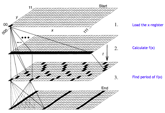
This tutorial deals with steps 2 and 3 of the algorithm, summarized mathematically below. The negative sign in the far right column vector is an accumulated phase due to the quantum Fourier transform.
\[ \frac{1}{ \sqrt{Q}} \sum_{x=0}^{Q-1} |x \rangle |f(x) \rangle = \frac{1}{2} \left[ \right] \xrightarrow{QFT} \frac{1}{2} \left[ \begin{pmatrix} 1 \\ 0 \\ 0 \\ 0 \end{pmatrix} \otimes \begin{pmatrix} 0 \\ 1 \\ 0 \\ 0 \\ 1 \end{pmatrix} + \begin{pmatrix} 0 \\ 0 \\ 1 \\ 0 \end{pmatrix} \otimes \begin{pmatrix} 0 \\ 1 \\ 0 \\ 0 \\ -1 \end{pmatrix} \right] \nonumber \]
How a Fourier transform on the x-register can yield the periodicity of f(x) which is on the y-register is revealed by carrying out the Fourier transform on the individual members of the x-register in the middle superposition term above.
\[ \frac{1}{2} \left[ \text{QFT} \begin{pmatrix} 1 \\ 0 \\ 0 \\ 0 \end{pmatrix} \begin{pmatrix} 0 \\ 1 \\ 0 \\ 0 \\ 0 \end{pmatrix} + \text{QFT} \begin{pmatrix} 0 \\ 1 \\ 0 \\ 0 \end{pmatrix} \begin{pmatrix} 0 \\ 0 \\ 0 \\ 0 \\ 1 \end{pmatrix} + \text{QFT} \begin{pmatrix} 0 \\ 0 \\ 1 \\ 0 \end{pmatrix} \begin{pmatrix} 0 \\ 1 \\ 0 \\ 0 \\ 0 \end{pmatrix} + \text{QFT} \begin{pmatrix} 0 \\ 0 \\ 0 \\ 1 \end{pmatrix} \begin{pmatrix} 0 \\ 0 \\ 0 \\ 0 \\ 1 \end{pmatrix} \right] \nonumber \]
\[ \begin{matrix} \text{QFT} \begin{pmatrix} 1 \\ 0 \\ 0 \\ 0 \end{pmatrix} = \begin{pmatrix} 0.5 \\ 0.5 \\ 0.5 \\ 0.5 \end{pmatrix} & \text{QFT} \begin{pmatrix} 0 \\ 1 \\ 0 \\ 0 \end{pmatrix} = \begin{pmatrix} 0.5 \\ 0.5i \\ -0.5 \\ -0.5i \end{pmatrix} & \text{QFT} \begin{pmatrix} 0 \\ 0 \\ 1 \\ 0 \end{pmatrix} = \begin{pmatrix} 0.5 \\ -0.5 \\ 0.5 \\ -0.5 \end{pmatrix} & \text{QFT} \begin{pmatrix} 0 \\ 0 \\ 0 \\ 1 \end{pmatrix} = \begin{pmatrix} 0.5 \\ -0.5i \\ -0.5 \\ 0.5i \end{pmatrix} \end{matrix} \nonumber \]
Using the results from (B) the QFT on the x-register in (A) yields the following superposition.
\[ \frac{1}{2} \left[ \frac{1}{2} \begin{pmatrix} 1 \\ 1 \\ 1 \\ 1 \end{pmatrix} \begin{pmatrix} 0 \\ 1 \\ 0 \\ 0 \\ 0 \end{pmatrix} + \frac{1}{2} \begin{pmatrix} 1 \\ i \\ -1 \\ -i \end{pmatrix} \begin{pmatrix} 0 \\ 0 \\ 0 \\ 0 \\ 1 \end{pmatrix} + \frac{1}{2} \begin{pmatrix} 1 \\ -1 \\ 1 \\ -1 \end{pmatrix} \begin{pmatrix} 0 \\ 1 \\ 0 \\ 0 \\ 0 \end{pmatrix} + \frac{1}{2} \begin{pmatrix} 1 \\ -i \\ -1 \\ i \end{pmatrix} \begin{pmatrix} 0 \\ 0 \\ 0 \\ 0 \\ 1 \end{pmatrix} \right] \nonumber \]
Constructive and destructive interference between the terms of this superposition leads to the final state.
\[ \frac{1}{2} \left[ \begin{pmatrix} 1 \\ 0 \\ 0 \\ 0 \end{pmatrix} \begin{pmatrix} 0 \\ 1 \\ 0 \\ 0 \\ 1 \end{pmatrix} + \begin{pmatrix} 0 \\ 0 \\ 1 \\ 0 \end{pmatrix} \begin{pmatrix} 0 \\ 1 \\ 0 \\ 0 \\ -1 \end{pmatrix} \right] \nonumber \]
The details of the interference between the terms in (C) can be seen by expanding them using vector tensor multiplication.
\[ \frac{1}{4} \left[ \begin{pmatrix} 0 \\ 1 \\ 0 \\ 0 \\ 0 \\ 0 \\ 1 \\ 0 \\ 0 \\ 0 \\ 0 \\ 1 \\ 0 \\ 0 \\ 0 \\ 0 \\ 1 \\ 0 \\ 0 \\ 0 \end{pmatrix} + \begin{pmatrix} 0 \\ 0 \\ 0 \\ 0 \\ 1 \\ 0 \\ 0 \\ 0 \\ 0 \\ i \\ 0 \\ 0 \\ 0 \\ 0 \\ -1 \\ 0 \\ 0 \\ 0 \\ 0 \\ -i \end{pmatrix} + \begin{pmatrix} 0 \\ 1 \\ 0 \\ 0 \\ 0 \\ 0 \\ -1 \\ 0 \\ 0 \\ 0 \\ 0 \\ 1 \\ 0 \\ 0 \\ 0 \\ 0 \\ -1 \\ 0 \\ 0 \\ 0 \end{pmatrix} + \begin{pmatrix} 0 \\ 0 \\ 0 \\ 0 \\ 1 \\ 0 \\ 0 \\ 0 \\ 0 \\ -i \\ 0 \\ 0 \\ 0 \\ 0 \\ -1 \\ 0 \\ 0 \\ 0 \\ 0 \\ i \end{pmatrix} \right] = \frac{1}{2} \begin{pmatrix} 0 \\ 1 \\ 0 \\ 0 \\ 1 \\ 0 \\ 0 \\ 0 \\ 0 \\ 0 \\ 0 \\ 1 \\ 0 \\ 0 \\ -1 \\ 0 \\ 0 \\ 0 \\ 0 \\ 0 \end{pmatrix} = \frac{1}{2} \left[ \begin{pmatrix} 1 \\ 0 \\ 0 \\ 0 \end{pmatrix} \begin{pmatrix} 0 \\ 1 \\ 0 \\ 0 \\ 1 \end{pmatrix} + \begin{pmatrix} 0 \\ 0 \\ 1 \\ 0 \end{pmatrix} \begin{pmatrix} 0 \\ 1 \\ 0 \\ 0 \\ -1 \end{pmatrix} \right] \nonumber \]
An algebraic view of (C) also reveals the x-register interference. Destructive interference occurs with the terms highlighted in red (|1>) and within the terms highlighted in blue (|3>).
\[ \begin{matrix} \frac{1}{4} \left[ |0 \rangle + |1 \rangle + |2 \rangle + |3 \rangle \right] |1 \rangle \\ + \\ \frac{1}{4} \left[ |0 \rangle + i |1 \rangle -|2 \rangle - i|3 \rangle \right] |4 \rangle \\ + & = \frac{1}{2} \left[ |0 \rangle \left( |1 \rangle + |4 \rangle \right) + |2 \rangle \left( |1 \rangle - |4 \rangle \right) \right] \\ \frac{1}{4} \left[ |0 \rangle -|1 \rangle + |2 \rangle - |3 \rangle \right] |1 \rangle \\ + \\ \frac{1}{4} \left[ |0 \rangle - i |1 \rangle - |2 \rangle + i|3 \rangle \right] |4 \rangle \end{matrix} \nonumber \]