8.80: Introduction to Superdense Coding

Quantum superdense coding reliably transmits two classical bits through an entangled pair of particles, even though only one member of the pair is handled by the sender. Charles Bennett, Physics Today, October 1995, p. 27

This tutorial is based on Brad Rubin's "Superdense Coding" at the Wolfram Demonstration Project: http:demonstrations.wolfram.com/SuperdenseCoding/. The quantum gate circuit shown below illustrates superdense coding, with Alice in control above the dotted line and Bob controlling the bottom part. Alice and Bob share the entangled pair of photons in the Bell basis shown at the left. Alice encodes two classical bits of information (four possible messages) on her photon, and Bob subsequently reads her message by performing a Bell state measurement on the modified entangled photon pair. In other words, although Alice encodes two bits on her photon Bob's readout requires a measurement involving both photons.

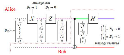
As shown above Alice and Bob share the following maximally entangled two-qubit state. It is easily recognized as one of four two-quibit Bell states.

\[ | \Phi_p \rangle = \frac{1}{ \sqrt{2}} \left[ |0 \rangle_A |0 \rangle_B + |1 \rangle_A + |1 \rangle_B \right] = \frac{1}{ \sqrt{2}} \left[ \begin{pmatrix} 1 \\ 0 \end{pmatrix} \otimes \begin{pmatrix} 1 \\ 0 \end{pmatrix} + \begin{pmatrix} 0 \\ 1 \end{pmatrix} \otimes \begin{pmatrix} 0 \\ 1 \end{pmatrix} \right] = \frac{1}{ \sqrt{2}} \begin{pmatrix} 1 \\ 0 \\ 0 \\ 1 \end{pmatrix} \nonumber \]

Before proceeding let's supplement the figure by showing how Alice and Bob might generate this state from an initial state in which they both possess |0> qubits.

\[ \begin{pmatrix} 1 \\ 0 \end{pmatrix} \otimes \begin{pmatrix} 1 \\ 0 \end{pmatrix} = \begin{pmatrix} 1 \\ 0 \\ 0 \\ 0 \end{pmatrix} \nonumber \]

This requires a Hadamard gate on the top wire followed by a two-qubit CNOT gate.

\[ \begin{matrix} I = \begin{pmatrix} 1 & 0 \\ 0 & 1 \end{pmatrix} & H = \frac{1}{ \sqrt{2}} \begin{pmatrix} 1 & 1 \\ 1 & -1 \end{pmatrix} & \text{CNOT} = \begin{pmatrix} 1 & 0 & 0 & 0 \\ 0 & 1 & 0 & 0 \\ 0 & 0 & 0 & 1 \\ 0 & 0 & 1 & 0 \end{pmatrix} & \text{CNOT kronecker(H, I)} \begin{pmatrix} 1 \\ 0 \\ 0 \\ 0 \end{pmatrix} = \begin{pmatrix} 0.707 \\ 0 \\ 0 \\ 0.707 \end{pmatrix} \end{matrix} \nonumber \]

Now the circuit in the figure is implemented using the Pauli gates (X and Z) on the top wire and controlled by Alice. Note on the right below that X⁰ and Z⁰ are the identity matrix (do nothing).

\[ \begin{matrix} \text{X} = \begin{pmatrix} 0 & 1 \\ 1 & 0 \end{pmatrix} & \text{Z} = \begin{pmatrix} 1 & 0 \\ 0 & -1 \end{pmatrix} & \text{X}^0 = \begin{pmatrix} 1 & 0 \\ 0 & 1 \end{pmatrix} & \text{Z}^0 = \begin{pmatrix} 1 & 0 \\ 0 & 1 \end{pmatrix} \end{matrix} \nonumber \]

\[ \begin{matrix} \text{Input} & \text{Output} \\ \text{B2= 0 B1 = 1 kronecker(H, I) CNOT kronecker} \left( Z^{B2},~ \text{I} \right) \text{kronecker} (X^{B1},~I) \frac{1}{ \sqrt{2}} \begin{pmatrix} 1 \\ 0 \\ 0 \\ 1 \end{pmatrix} = \begin{pmatrix} 0 \\ 1 \\ 0 \\ 0 \end{pmatrix} & \text{B2 B1} = \begin{pmatrix} 1 \\ 0 \end{pmatrix} \begin{pmatrix} 0 \\ 1 \end{pmatrix} = \begin{pmatrix} 0 \\ 1 \\ 0 \\ 0 \end{pmatrix} \end{matrix} \nonumber \]

Next we do the same for the other classical two-bit states.

\[ \begin{matrix} \text{B2= 0 B1 = 0 kronecker(H, I) CNOT kronecker} \left( Z^{B2},~ \text{I} \right) \text{kronecker} (X^{B1},~I) \frac{1}{ \sqrt{2}} \begin{pmatrix} 1 \\ 0 \\ 0 \\ 1 \end{pmatrix} = \begin{pmatrix} 1 \\ 0 \\ 0 \\ 0 \end{pmatrix} & \text{B2 B1} = \begin{pmatrix} 1 \\ 0 \end{pmatrix} \begin{pmatrix} 0 \\ 1 \end{pmatrix} = \begin{pmatrix} 1 \\ 0 \\ 0 \\ 0 \end{pmatrix} \\ \text{B2= 0 B1 = 0 kronecker(H, I) CNOT kronecker} \left( Z^{B2},~ \text{I} \right) \text{kronecker} (X^{B1},~I) \frac{1}{ \sqrt{2}} \begin{pmatrix} 1 \\ 0 \\ 0 \\ 1 \end{pmatrix} = \begin{pmatrix} 0 \\ 0 \\ 1 \\ 0 \end{pmatrix} & \text{B2 B1} = \begin{pmatrix} 1 \\ 0 \end{pmatrix} \begin{pmatrix} 0 \\ 1 \end{pmatrix} = \begin{pmatrix} 0 \\ 0 \\ 1 \\ 0 \end{pmatrix} \\ \text{B2= 1 B1 = 0 kronecker(H, I) CNOT kronecker} \left( Z^{B2},~ \text{I} \right) \text{kronecker} (X^{B1},~I) \frac{1}{ \sqrt{2}} \begin{pmatrix} 1 \\ 0 \\ 0 \\ 1 \end{pmatrix} = \begin{pmatrix} 0 \\ 0 \\ 0 \\ 1 \end{pmatrix} & \text{B2 B1} = \begin{pmatrix} 1 \\ 0 \end{pmatrix} \begin{pmatrix} 0 \\ 1 \end{pmatrix} = \begin{pmatrix} 0 \\ 0 \\ 0 \\ 1 \end{pmatrix} \end{matrix} \nonumber \]

Of course we could have done all this starting with the |0>A|0>B state as is shown below using B2 and B1 from the last example. Note the mirror symmetry involving the beginning and end of this quantum gate circuit. It begins by creating a Bell state and ends by making a Bell state measurement. In between, depending on the values of B1 and B2, the initial Bell state is transformed by X and Z in steps into a final Bell state which is measured. This will be demonstrated below.

\[ \text{kronecker(H, I) CNOT kronecker} \left( Z^{B2},~I \right) \text{kronecker} \left( X^{B1},~I \right) \text{CNOT kronecker(H, I)} \begin{pmatrix} 1 \\ 0 \\ 0 \\ 0 \end{pmatrix} = \begin{pmatrix} 0 \\ 0 \\ 0 \\ 1 \end{pmatrix} \nonumber \]

Bell states:

\[ \begin{matrix} \Phi_p = \frac{1}{ \sqrt{2}} \begin{pmatrix} 1 \\ 0 \\ 0 \\ 1 \end{pmatrix} & \Phi_m = \frac{1}{ \sqrt{2}} \begin{pmatrix} 1 \\ 0 \\ 0 \\ -1 \end{pmatrix} & \Psi_p = \frac{1}{ \sqrt{2}} \begin{pmatrix} 0 \\ 1 \\ 1 \\ 0 \end{pmatrix} & \Psi_m = \frac{1}{ \sqrt{2}} \begin{pmatrix} 0 \\ 1 \\ -1 \\ 0 \end{pmatrix} \end{matrix} \nonumber \]

\[ \begin{matrix} ~ & \text{Step1} & ~ & ~ & \text{Step 2} & ~ & ~ & \text{Measure} \\ \text{B2 = 0 B1 = 0} & \Phi_p & \Phi_p & ~ & \Phi_p & \Phi_p & ~ & \Phi_p \\ \text{kronecker} \left( X^{B1},~ \text{I} \right) \frac{1}{ \sqrt{2}} & \begin{pmatrix} 1 \\ 0 \\ 0 \\ 1 \end{pmatrix} = & \begin{pmatrix} 0.707 \\ 0 \\ 0 \\ 0.707 \end{pmatrix} & \text{kronecker} \left( Z^{B2},~I \right) & \begin{pmatrix} 0.707 \\ 0 \\ 0 \\ 0.707 \end{pmatrix} = & \begin{pmatrix} 0.707 \\ 0 \\ 0 \\ 0.707 \end{pmatrix} & \text{kronecker(H, I) CNOT} & \begin{pmatrix} 0.707 \\ 0 \\ 0 \\ 0.707 \end{pmatrix} = & \begin{pmatrix} 1 \\ 0 \\ 0 \\ 0 \end{pmatrix} \end{matrix} \nonumber \]

\[ \begin{matrix} \cdot & \fbox{X}^0 & \cdot & \fbox{Z}^0 & \cdot & \cdot & \fbox{H} & \cdot \\ \begin{pmatrix} \frac{1}{ \sqrt{2}} \\ 0 \\ 0 \\ \frac{1}{ \sqrt{2}} \end{pmatrix} & ~ & \begin{pmatrix} \frac{1}{ \sqrt{2}} \\ 0 \\ 0 \\ \frac{1}{ \sqrt{2}} \end{pmatrix} & ~ & \begin{pmatrix} \frac{1}{ \sqrt{2}} \\ 0 \\ 0 \\ \frac{1}{ \sqrt{2}} \end{pmatrix} & \begin{matrix} | \\ | \\ | \\ | \end{matrix} & ~ & \begin{pmatrix} 1 \\ 0 \\ 0 \\ 0 \end{pmatrix} = \begin{pmatrix} 1 \\ 0 \end{pmatrix} \begin{pmatrix} 1 \\ 0 \end{pmatrix} = |0 \rangle \\ \cdot & \cdots & \cdot & \cdots & \cdot & \oplus & \cdots & \cdot \end{matrix} \nonumber \]

\[ \frac{|00 \rangle + |11 \rangle}{ \sqrt{2}} \xrightarrow{X^0 \oplus I} \frac{|00 \rangle +|11 \rangle}{ \sqrt{2}} \xrightarrow{Z^0 \otimes I} \frac{|00 \rangle + |11 \rangle}{ \sqrt{2}} \xrightarrow{ \text{CNOT}} \frac{|00 \rangle +|10 \rangle}{ \sqrt{2}} \xrightarrow{H \otimes I} \frac{(|0 \rangle +|1 \rangle) |0 \rangle + (|0 \rangle - |1 \rangle ) |0 \rangle}{ \sqrt{2}} = |00 \rangle = |0 \rangle \nonumber \]

\[ \begin{matrix} \text{B2 = 0 B1 = 1} & \Phi_p & \Psi_p & ~ & \Psi_p & \Psi_p & ~ & \Psi_p \\ \text{kronecker} \left( X^{B1},~ \text{I} \right) \frac{1}{ \sqrt{2}} & \begin{pmatrix} 1 \\ 0 \\ 0 \\ 1 \end{pmatrix} = & \begin{pmatrix} 0 \\ 0.707 \\ 0.707 \\ 0 \end{pmatrix} & \text{kronecker} \left( Z^{B2},~I \right) & \begin{pmatrix} 0 \\ 0.707 \\ 0.707 \\ 0 \end{pmatrix} = & \begin{pmatrix} 0 \\ 0.707 \\ 0.707 \\ 0 \end{pmatrix} & \text{kronecker(H, I) CNOT} & \begin{pmatrix} 0 \\ 0.707 \\ 0.707 \\ 0 \end{pmatrix} = & \begin{pmatrix} 0 \\ 1 \\ 0 \\ 0 \end{pmatrix} \end{matrix} \nonumber \]

\[ \begin{matrix} \cdot & \fbox{X}^1 & \cdot & \fbox{Z}^0 & \cdot & \cdot & \fbox{H} & \cdot \\ \begin{pmatrix} \frac{1}{ \sqrt{2}} \\ 0 \\ 0 \\ \frac{1}{ \sqrt{2}} \end{pmatrix} & ~ & \begin{pmatrix} ~ \\ \frac{1}{ \sqrt{2}} \\ \frac{1}{ \sqrt{2}} \\ 0 \end{pmatrix} & ~ & \begin{pmatrix} ~ \\ \frac{1}{ \sqrt{2}} \\ \frac{1}{ \sqrt{2}} \\ 0 \end{pmatrix} & \begin{matrix} | \\ | \\ | \\ | \end{matrix} & ~ & \begin{pmatrix} 0 \\ 1 \\ 0 \\ 0 \end{pmatrix} = \begin{pmatrix} 1 \\ 0 \end{pmatrix} \begin{pmatrix} 0 \\ 1 \end{pmatrix} = |1 \rangle \\ \cdot & \cdots & \cdot & \cdots & \cdot & \oplus & \cdots & \cdot \end{matrix} \nonumber \]

\[ \frac{|00 \rangle + |11 \rangle}{ \sqrt{2}} \xrightarrow{X \oplus I} \frac{|10 \rangle +|01 \rangle}{ \sqrt{2}} \xrightarrow{Z^0 \otimes I} \frac{|10 \rangle + |01 \rangle}{ \sqrt{2}} \xrightarrow{ \text{CNOT}} \frac{|11 \rangle +|01 \rangle}{ \sqrt{2}} \xrightarrow{H \otimes I} \frac{(|0 \rangle -|1 \rangle) |1 \rangle + (|0 \rangle + |1 \rangle ) |1 \rangle}{ \sqrt{2}} = |01 \rangle = |1 \rangle \nonumber \]

\[ \begin{matrix} \text{B2 = 1 B1 = 0} & \Phi_p & \Phi_p & ~ & \Phi_p & \Phi_m & ~ & \Phi_m \\ \text{kronecker} \left( X^{B1},~ \text{I} \right) \frac{1}{ \sqrt{2}} & \begin{pmatrix} 1 \\ 0 \\ 0 \\ 1 \end{pmatrix} = & \begin{pmatrix} 0.707 \\ 0 \\ 0 \\ 0.707 \end{pmatrix} & \text{kronecker} \left( Z^{B2},~I \right) & \begin{pmatrix} 0.707 \\ 0 \\ 0 \\ 0.707 \end{pmatrix} = & \begin{pmatrix} 0.707 \\ 0 \\ 0 \\ -0.707 \end{pmatrix} & \text{kronecker(H, I) CNOT} & \begin{pmatrix} 0.707 \\ 0 \\ 0 \\ -0.707 \end{pmatrix} = & \begin{pmatrix} 0 \\ 0 \\ 1 \\ 0 \end{pmatrix} \end{matrix} \nonumber \]

\[ \begin{matrix} \cdot & \fbox{X}^0 & \cdot & \fbox{Z}^1 & \cdot & \cdot & \fbox{H} & \cdot \\ \begin{pmatrix} \frac{1}{ \sqrt{2}} \\ 0 \\ 0 \\ \frac{1}{ \sqrt{2}} \end{pmatrix} & ~ & \begin{pmatrix} \frac{1}{ \sqrt{2}} \\ 0 \\ 0 \\ \frac{1}{ \sqrt{2}} \end{pmatrix} & ~ & \begin{pmatrix} \frac{1}{ \sqrt{2}} \\ 0 \\ 0 \\ - \frac{1}{ \sqrt{2}} \end{pmatrix} & \begin{matrix} | \\ | \\ | \\ | \end{matrix} & ~ & \begin{pmatrix} 0 \\ 0 \\ 1 \\ 0 \end{pmatrix} = \begin{pmatrix} 0 \\ 1 \end{pmatrix} \begin{pmatrix} 1 \\ 0 \end{pmatrix} = |2 \rangle \\ \cdot & \cdots & \cdot & \cdots & \cdot & \oplus & \cdots & \cdot \end{matrix} \nonumber \]

\[ \frac{|00 \rangle + |11 \rangle}{ \sqrt{2}} \xrightarrow{X^0 \oplus I} \frac{|00 \rangle +|11 \rangle}{ \sqrt{2}} \xrightarrow{Z^0 \otimes I} \frac{|00 \rangle - |11 \rangle}{ \sqrt{2}} \xrightarrow{ \text{CNOT}} \frac{|00 \rangle - |10 \rangle}{ \sqrt{2}} \xrightarrow{H \otimes I} \frac{(|0 \rangle +|1 \rangle) |0 \rangle + (|0 \rangle - |1 \rangle ) |0 \rangle}{ \sqrt{2}} = |10 \rangle = |2 \rangle \nonumber \]

\[ \begin{matrix} \text{B2 = 1 B1 = 1} & \Phi_p & \Phi_p & ~ & \Psi_p & \Psi_m & ~ & \Psi_m \\ \text{kronecker} \left( X^{B1},~ \text{I} \right) \frac{1}{ \sqrt{2}} & \begin{pmatrix} 1 \\ 0 \\ 0 \\ 1 \end{pmatrix} = & \begin{pmatrix} 0 \\ 0.707 \\ 0.707 \\ 0 \end{pmatrix} & \text{kronecker} \left( Z^{B2},~I \right) & \begin{pmatrix} 0 \\ 0.707 \\ 0.707 \\ 0 \end{pmatrix} = & \begin{pmatrix} 0 \\ 0.707 \\ -0.707 \\ 0 \end{pmatrix} & \text{kronecker(H, I) CNOT} & \begin{pmatrix} 0 \\ 0.707 \\ -0.707 \\ 0 \end{pmatrix} = & \begin{pmatrix} 0 \\ 0 \\ 0 \\ 1 \end{pmatrix} \end{matrix} \nonumber \]

\[ \begin{matrix} \cdot & \fbox{X}^1 & \cdot & \fbox{Z}^1 & \cdot & \cdot & \fbox{H} & \cdot \\ \begin{pmatrix} \frac{1}{ \sqrt{2}} \\ 0 \\ 0 \\ \frac{1}{ \sqrt{2}} \end{pmatrix} & ~ & \begin{pmatrix} ~ \\ \frac{1}{ \sqrt{2}} \\ \frac{1}{ \sqrt{2}} \\ 0 \end{pmatrix} & ~ & \begin{pmatrix} ~ \\ \frac{1}{ \sqrt{2}} \\ - \frac{1}{ \sqrt{2}} \\ 0 \end{pmatrix} & \begin{matrix} | \\ | \\ | \\ | \end{matrix} & ~ & \begin{pmatrix} 0 \\ 0 \\ 0 \\ 1 \end{pmatrix} = \begin{pmatrix} 0 \\ 1 \end{pmatrix} \begin{pmatrix} 0 \\ 1 \end{pmatrix} = |3 \rangle \\ \cdot & \cdots & \cdot & \cdots & \cdot & \oplus & \cdots & \cdot \end{matrix} \nonumber \]

\[ \frac{|00 \rangle + |11 \rangle}{ \sqrt{2}} \xrightarrow{X^0 \oplus I} \frac{|10 \rangle +|01 \rangle}{ \sqrt{2}} \xrightarrow{Z^0 \otimes I} \frac{ -|10 \rangle + |01 \rangle}{ \sqrt{2}} \xrightarrow{ \text{CNOT}} \frac{ -|11 \rangle + |01 \rangle}{ \sqrt{2}} \xrightarrow{H \otimes I} \frac{-(|0 \rangle -|1 \rangle) |1 \rangle + (|0 \rangle + |1 \rangle ) |1 \rangle}{ \sqrt{2}} = |11 \rangle = |3 \rangle \nonumber \]

It is now shown that steps 1 and 2 in the original calculation can be condensed into one step.

\[ \begin{matrix} \text{Binary Input} & ~ & \text{Binary Bell State Index} & \text{Decimal Bell State Intex} \\ \text{B2 = 0 B1 = 0} & \text{kronecker(H, I) CNOT kronecker} \left( Z^{B2}X^{B1},~ \text{I} \right) \Psi_p = \begin{pmatrix} 1 \\ 0 \\ 0 \\ 0 \end{pmatrix} & |00 \rangle & |0 \rangle \\ \text{B2 = 0 B1 = 1} & \text{kronecker(H, I) CNOT kronecker} \left( Z^{B2}X^{B1},~ \text{I} \right) \Psi_p = \begin{pmatrix} 0 \\ 1 \\ 0 \\ 0 \end{pmatrix} & |01 \rangle & |1 \rangle \\ \text{B2 = 1 B1 = 0} & \text{kronecker(H, I) CNOT kronecker} \left( Z^{B2}X^{B1},~ \text{I} \right) \Psi_p = \begin{pmatrix} 0 \\ 0 \\ 1 \\ 0 \end{pmatrix} & |10 \rangle & |2 \rangle \\ \text{B2 = 1 B1 = 1} & \text{kronecker(H, I) CNOT kronecker} \left( Z^{B2}X^{B1},~ \text{I} \right) \Psi_p = \begin{pmatrix} 0 \\ 0 \\ 0 \\ 1 \end{pmatrix} & |11 \rangle & |3 \rangle \end{matrix} \nonumber \]