8.76: Implementation of Deutsch's Algorithm Using Mathcad

The following is a Mathcad implementation of David Deutsch's quantum computer prototype as presented on pages 10-11 in "Machines, Logic and Quantum Physics" by David Deutsch, Artur Ekert, and Rossella Lupacchini, which can be found at arXiv:math.HO/9911150v1.

A function f maps {0, 1} to {0, 1}. There are four possible outcomes: f(0) = 0; f(0) = 1; f(1) = 0; f(1) = 1. The task Deutsch tackled was to develop an implementable quantum algorithm which could determine whether f(0) and f(1) were the same or different in a single calculation. By comparison classical computers require two calculations for such a task - calculating both f(0) and f(1) to see if they are the same or different.

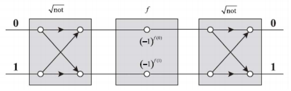
The proposed quantum computer consists of three one-qubit gates in the arrangement shown below. The \( \sqrt{NOT}\) gates are 50-50 beam splitters that assign a π/2 (i, 90 degree) phase change to reflection relative to transmission. For example, the first gate creates the following superpositions of the inputs |0> and |1>.

\[ \begin{matrix} |0 \rangle \rightarrow \left[ |0 \rangle + i|1 \rangle \right] & |1 \rangle \rightarrow \left[ i|0 \rangle + |1 \rangle \right] \end{matrix} \nonumber \]

The middle gate carries out phase shifts on the superposition created by the first gate. Depending on the f-values, the operation of the second \( \sqrt{NOT}\) converts the superposition to either |0> or |1> multiplied by a phase factor or unity. The Deutsch circuit is essentially a two-port Mach-Zehnder interferometer with the possibility for unequal phase changes in its upper and lower arms.

The matrix representations for the gates are as follows:

\[ \begin{matrix} 0 = \begin{pmatrix} 1 \\ 0 \end{pmatrix} & ~ & ~ & ~ & 0 = \begin{pmatrix} 1 \\ 0 \end{pmatrix} \\ ~ & \frac{1}{ \sqrt{2}} \begin{pmatrix} 1 & i \\ i & 1 \end{pmatrix} & \begin{bmatrix} (-1)^{f(0)} & 0 \\ 0 & (-1)^{f(1)} \end{bmatrix} & \frac{1}{ \sqrt{2}} \begin{pmatrix} 1 & i \\ i & 1 \end{pmatrix} & ~ \\ 1 = \begin{pmatrix} 0 \\ 1 \end{pmatrix} & ~ & ~ & ~ & 1 = \begin{pmatrix} 0 \\ 1 \end{pmatrix} \end{matrix} \nonumber \]

We begin with a matrix mechanics approach to Deutsch's algorithm using the definitions provided immediately above. There are two input ports and two output ports, but only one input port is used in any given computational run. First it is shown how the output result depends on the input port chosen in terms of the values of f(0) and f(1).

\[ \begin{matrix} \begin{pmatrix} 1 \\ 0 \end{pmatrix} ~ \text{Input} & \left[ \frac{1}{ \sqrt{2}} \begin{pmatrix} 1 & i \\ i & 1 \end{pmatrix} \right] \begin{bmatrix} (-1)^{f_0} & 0 \\ 0 & (-1)^{f_1} \end{bmatrix} \left[ \frac{1}{ \sqrt{2}} \begin{pmatrix} 1 & i \\ i & 1 \end{pmatrix} \right] \begin{pmatrix} 1 \\ 0 \end{pmatrix} \rightarrow \begin{bmatrix} \frac{(-1)^{f_0}}{2} - \frac{(-1)^{f_1}}{2} \\ \frac{(-1)^f_0}{2} + \frac{(-1)^{f_1} i}{2} \end{bmatrix} \\ \begin{pmatrix} 0 \\ 1 \end{pmatrix} ~ \text{Input} & \left[ \frac{1}{ \sqrt{2}} \begin{pmatrix} 1 & i \\ i & 1 \end{pmatrix} \right] \begin{bmatrix} (-1)^{f_0} & 0 \\ 0 & (-1)^{f_1} \end{bmatrix} \left[ \frac{1}{ \sqrt{2}} \begin{pmatrix} 1 & i \\ i & 1 \end{pmatrix} \right] \begin{pmatrix} 0 \\ 1 \end{pmatrix} \rightarrow \begin{bmatrix} \frac{(-1)^f_0}{2} + \frac{(-1)^{f_1} i}{2} \\ \frac{(-1)^{f_0}}{2} - \frac{(-1)^{f_1}}{2} \end{bmatrix} \end{matrix} \nonumber \]

These calculations and the circuit diagram show that there are two paths to each output port from each input port. As will now be shown these paths interfere constructively or destructively depending on the phase changes brought about by the middle circuit element's values of f(0) and f(1).

The following calculations show that the probability that |0 > input leads to |0 > output is zero if f(0) and f(1) are the same (both 0 or both 1), and unity if they are different (one 0, the other 1). Thus the task has been successfully accomplished. The highlighted central region calculates the output state for input state |0> given the values of f(0) and f(1) to the left. On the right the probability that |0> is the output state is calculated.

\[ \begin{matrix} f_0 = 0 & f_1 = 0 & \left[ \frac{1}{ \sqrt{2}} \begin{pmatrix} 1 & i \\ i & 1 \end{pmatrix} \right] \begin{bmatrix} (-1)^{f_0} & 0 \\ 0 & (-1)^{f_1} \end{bmatrix} \left[ \frac{1}{ \sqrt{2}} \begin{pmatrix} 1 & i \\ i & 1 \end{pmatrix} \right] \begin{pmatrix} 1 \\ 0 \end{pmatrix} = \begin{pmatrix} 0 \\ i \end{pmatrix} & \left[ \left| \begin{pmatrix} 1 & 0 \end{pmatrix} \begin{pmatrix} 0 \\ i \end{pmatrix} \right| \right]^2 = 0 \\ f_0 = 1 & f_1 = 1 & \left[ \frac{1}{ \sqrt{2}} \begin{pmatrix} 1 & i \\ i & 1 \end{pmatrix} \right] \begin{bmatrix} (-1)^{f_0} & 0 \\ 0 & (-1)^{f_1} \end{bmatrix} \left[ \frac{1}{ \sqrt{2}} \begin{pmatrix} 1 & i \\ i & 1 \end{pmatrix} \right] \begin{pmatrix} 1 \\ 0 \end{pmatrix} = \begin{pmatrix} 0 \\ -i \end{pmatrix} & \left[ \left| \begin{pmatrix} 1 & 0 \end{pmatrix} \begin{pmatrix} 0 \\ -i \end{pmatrix} \right| \right]^2 = 0 \\ f_0 = 1 & f_1 = 0 & \left[ \frac{1}{ \sqrt{2}} \begin{pmatrix} 1 & i \\ i & 1 \end{pmatrix} \right] \begin{bmatrix} (-1)^{f_0} & 0 \\ 0 & (-1)^{f_1} \end{bmatrix} \left[ \frac{1}{ \sqrt{2}} \begin{pmatrix} 1 & i \\ i & 1 \end{pmatrix} \right] \begin{pmatrix} 1 \\ 0 \end{pmatrix} = \begin{pmatrix} -1 \\ 0 \end{pmatrix} & \left[ \left| \begin{pmatrix} 1 & 0 \end{pmatrix} \begin{pmatrix} -1 \\ 0 \end{pmatrix} \right| \right]^2 = 1 \\ f_0 = 0 & f_1 = 1 & \left[ \frac{1}{ \sqrt{2}} \begin{pmatrix} 1 & i \\ i & 1 \end{pmatrix} \right] \begin{bmatrix} (-1)^{f_0} & 0 \\ 0 & (-1)^{f_1} \end{bmatrix} \left[ \frac{1}{ \sqrt{2}} \begin{pmatrix} 1 & i \\ i & 1 \end{pmatrix} \right] \begin{pmatrix} 1 \\ 0 \end{pmatrix} = \begin{pmatrix} 1 \\ 0 \end{pmatrix} & \left[ \left| \begin{pmatrix} 1 & 0 \end{pmatrix} \begin{pmatrix} 1 \\ 0 \end{pmatrix} \right| \right]^2 = 1 \end{matrix} \nonumber \]

As might be expected, similar calculations show that the probability that |1> input leads to |1> output is zero if f(0) and f(1) are the same, and unity if they are different.

\[ \begin{matrix} f_0 = 0 & f_1 = 0 & \left[ \frac{1}{ \sqrt{2}} \begin{pmatrix} 1 & i \\ i & 1 \end{pmatrix} \right] \begin{bmatrix} (-1)^{f_0} & 0 \\ 0 & (-1)^{f_1} \end{bmatrix} \left[ \frac{1}{ \sqrt{2}} \begin{pmatrix} 1 & i \\ i & 1 \end{pmatrix} \right] \begin{pmatrix} 0 \\ 1 \end{pmatrix} = \begin{pmatrix} i \\ 0 \end{pmatrix} & \left[ \left| \begin{pmatrix} 0 & 1 \end{pmatrix} \begin{pmatrix} i \\ 0 \end{pmatrix} \right| \right]^2 = 0 \\ f_0 = 1 & f_1 = 1 & \left[ \frac{1}{ \sqrt{2}} \begin{pmatrix} 1 & i \\ i & 1 \end{pmatrix} \right] \begin{bmatrix} (-1)^{f_0} & 0 \\ 0 & (-1)^{f_1} \end{bmatrix} \left[ \frac{1}{ \sqrt{2}} \begin{pmatrix} 1 & i \\ i & 1 \end{pmatrix} \right] \begin{pmatrix} 0 \\ 1 \end{pmatrix} = \begin{pmatrix} -i \\ 0 \end{pmatrix} & \left[ \left| \begin{pmatrix} 0 & 1 \end{pmatrix} \begin{pmatrix} -i \\ 0 \end{pmatrix} \right| \right]^2 = 0 \\ f_0 = 1 & f_1 = 0 & \left[ \frac{1}{ \sqrt{2}} \begin{pmatrix} 1 & i \\ i & 1 \end{pmatrix} \right] \begin{bmatrix} (-1)^{f_0} & 0 \\ 0 & (-1)^{f_1} \end{bmatrix} \left[ \frac{1}{ \sqrt{2}} \begin{pmatrix} 1 & i \\ i & 1 \end{pmatrix} \right] \begin{pmatrix} 0 \\ 1 \end{pmatrix} = \begin{pmatrix} 0 \\ 1 \end{pmatrix} & \left[ \left| \begin{pmatrix} 0 & 1 \end{pmatrix} \begin{pmatrix} 0 \\ 1 \end{pmatrix} \right| \right]^2 = 1 \\ f_0 = 0 & f_1 = 1 & \left[ \frac{1}{ \sqrt{2}} \begin{pmatrix} 1 & i \\ i & 1 \end{pmatrix} \right] \begin{bmatrix} (-1)^{f_0} & 0 \\ 0 & (-1)^{f_1} \end{bmatrix} \left[ \frac{1}{ \sqrt{2}} \begin{pmatrix} 1 & i \\ i & 1 \end{pmatrix} \right] \begin{pmatrix} 0 \\ 1 \end{pmatrix} = \begin{pmatrix} 0 \\ -1 \end{pmatrix} & \left[ \left| \begin{pmatrix} 0 & 1 \end{pmatrix} \begin{pmatrix} 0 \\ -1 \end{pmatrix} \right| \right]^2 = 1 \end{matrix} \nonumber \]

Examination of the Deutsch circuit reveals certain similarities with the double-slit experiment. For example, there are two paths for input |0> to output |0> and input |1> to output |1> (and also for |0> --> |1> and |1> --> |0>, but they are not of interest here). As Deutsch and his co-authors state, this is the secret of the quantum computer - the possibility of constructive and destructive interference of the probability amplitudes for the various computational paths.

Addition of probability amplitudes, rather than probabilities, is one of the fundamental rules for prediction in quantum mechanics and applies to all physical objects, in particular quantum computing machines. If a computing machine starts in a specific initial configuration (input) then the probability that after its evolution via a sequence of intermediate configurations it ends up in a specific final configuration (output) is the squared modulus of the sum of all the probability amplitudes of the computational paths that connect the input with the output. The amplitudes are complex numbers and may cancel each other, which is referred to as destructive interference, or enhance each other, referred to as constructive interference. The basic idea of quantum computation is to use quantum interference to amplify the correct outcomes and to suppress the incorrect outcomes of computations.

Recall from above (see the matrix representing the \( \sqrt{NOT}\) beam splitters) that the probability amplitude for transmission at the beam splitters is \( \frac{1}{ \sqrt{2}}\), and the probability amplitude for reflection is \( \frac{i}{ \sqrt{2}}\). The middle element of the circuit causes phase shifts on its input wires that depend on the values of f(0) and f(1). From the circuit diagram we see that |0> output from |0> input can be achieved by two transmissions and a phase shift on the upper wire or reflection to the lower wire, phase shift, followed by reflection to the upper wire. The absolute magnitude squared of the sum of these probability amplitudes is calculated for the four possible values for f(0) and f(1).

\[ \begin{matrix} f_0 = 0 & f_1 = 0 & \left[ \left| \frac{1}{ \sqrt{2}} (-1)^{f_0} \frac{1}{ \sqrt{2}} + \frac{1}{ \sqrt{2}} (-1)^{f_1} \frac{i}{ \sqrt{2}} \right| \right]^2 = 0 \\ f_0 = 1 & f_1 = 1 & \left[ \left| \frac{1}{ \sqrt{2}} (-1)^{f_0} \frac{1}{ \sqrt{2}} + \frac{1}{ \sqrt{2}} (-1)^{f_1} \frac{i}{ \sqrt{2}} \right| \right]^2 = 0 \\ f_0 = 1 & f_1 = 0 & \left[ \left| \frac{1}{ \sqrt{2}} (-1)^{f_0} \frac{1}{ \sqrt{2}} + \frac{1}{ \sqrt{2}} (-1)^{f_1} \frac{i}{ \sqrt{2}} \right| \right]^2 = 1 \\ f_0 = 0 & f_1 = 1 & \left[ \left| \frac{1}{ \sqrt{2}} (-1)^{f_0} \frac{1}{ \sqrt{2}} + \frac{1}{ \sqrt{2}} (-1)^{f_1} \frac{i}{ \sqrt{2}} \right| \right]^2 = 1 \end{matrix} \nonumber \]

As expected we see consistency with the previous calculations. However, this method has the advantage of more directly revealing what is happening from the quantum mechanical perspective. When f(0) and f(1) are the same the two path amplitudes interfere destructively; when they are different there is constructive interference between the path amplitudes.

As can be seen from above, in the absence of the middle element of the quantum circuit, the two paths from |0> to |0> are 180 degrees out of phase and therefore destructively interfere. In the presence of the middle element the paths are still 180 degrees out of phase unless the f-values are different, and then they are brought into phase and constructively interfere.

As Feynman emphasized in his eponymous lecture series on physics, the creation of superpositions and the interference of probability amplitudes are the essence of quantum mechanics.

Another implementation of Deutsch's algorithm is due to Artur Ekert and co-workers (see Julian Brown's The Quest for the Quantum Computer, pages 353-355).

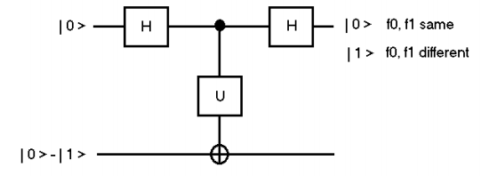
The following table provides a summary of the results. If qubit 1 is |0> f(0) and f(1) are the same, but if it is |1> they are different.

\[ \begin{bmatrix} f_0 & 0 & 1 & 1 & 0 \\ f_1 & 0 & 1 & 0 & 1 \\ \text{qubit1} & \begin{pmatrix} 1 \\ 0 \end{pmatrix} & \begin{pmatrix} 1 \\ 0 \end{pmatrix} & \begin{pmatrix} 0 \\ 1 \end{pmatrix} & \begin{pmatrix} 0 \\ 1 \end{pmatrix} \\ \text{qubit2} & \begin{pmatrix} -0.707 \\ 0.707 \end{pmatrix} & \begin{pmatrix} 0.707 \\ -0.707 \end{pmatrix} & \begin{pmatrix} 0.707 \\ -0.707 \end{pmatrix} & \begin{pmatrix} -0.707 \\ 0.707 \end{pmatrix} \\ \text{OutputState} & \begin{pmatrix} -0.707 \\ 0.707 \\ 0 \\ 0 \end{pmatrix} & \begin{pmatrix} 0.707 \\ -0.707 \\ 0 \\ 0 \end{pmatrix} & \begin{pmatrix} 0 \\ 0 \\ 0.707 \\ -0.707 \end{pmatrix} & \begin{pmatrix} 0 \\ 0 \\ -0.707 \\ 0.707 \end{pmatrix} \end{bmatrix} \nonumber \]

The algorithm is implemented below.

\[ \begin{matrix} \text{Identity} & \text{I} = \begin{pmatrix} 1 & 0 \\ 0 & 1 \end{pmatrix} & \text{Not gate:} & \text{NOT} = \begin{pmatrix} 0 & 1 \\ 1 & 0 \end{pmatrix} & \text{Hadamard gate:} & \text{H} = \frac{1}{ \sqrt{2}} \begin{pmatrix} 1 & 1 \\ 1 & -1 \end{pmatrix} \end{matrix} \nonumber \]

\[ \begin{matrix} f_0 = 0 & f_1 = 0 & \text{kronecker(H, I) kronecker} \left[ \begin{bmatrix} (-1)^{f_0} & 0 \\ 0 & (-1)^{f_1} \end{bmatrix},~ \text{NOT} \right] \text{kronecker(H, I) } \frac{1}{ \sqrt{2}} \begin{pmatrix} 1 \\ -1 \\ 0 \\ 0 \end{pmatrix} = \begin{pmatrix} -0.707 \\ 0.707 \\ 0 \\ 0 \end{pmatrix} \\ f_0 = 1 & f_1 = 1 & \text{kronecker(H, I) kronecker} \left[ \begin{bmatrix} (-1)^{f_0} & 0 \\ 0 & (-1)^{f_1} \end{bmatrix},~ \text{NOT} \right] \text{kronecker(H, I)} \frac{1}{ \sqrt{2}} \begin{pmatrix} 1 \\ -1 \\ 0 \\ 0 \end{pmatrix} = \begin{pmatrix} 0.707 \\ -0.707 \\ 0 \\ 0 \end{pmatrix} \\ f_0 = 1 & f_1 = 0 & \text{kronecker(H, I) kronecker} \left[ \begin{bmatrix} (-1)^{f_0} & 0 \\ 0 & (-1)^{f_1} \end{bmatrix},~ \text{NOT} \right] \text{kronecker(H, I)} \frac{1}{ \sqrt{2}} \begin{pmatrix} 1 \\ -1 \\ 0 \\ 0 \end{pmatrix} = \begin{pmatrix} 0 \\ 0 \\ 0.707 \\ -0.707 \end{pmatrix} \\ f_0 = 0 & f_1 = 1 & \text{kronecker(H, I) kronecker} \left[ \begin{bmatrix} (-1)^{f_0} & 0 \\ 0 & (-1)^{f_1} \end{bmatrix},~ \text{NOT} \right] \text{kronecker(H, I)} \frac{1}{ \sqrt{2}} \begin{pmatrix} 1 \\ -1 \\ 0 \\ 0 \end{pmatrix} = \begin{pmatrix} 0 \\ 0 \\ -0.707 \\ 0.707 \end{pmatrix} \end{matrix} \nonumber \]

It is easy to show that the output of each of these calculations is the tensor product of qubits 1 and 2 in the summary table provided above.

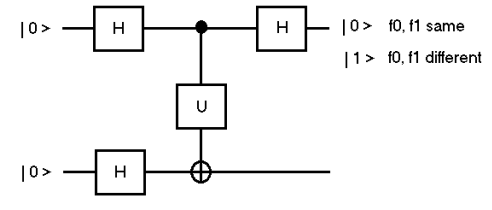
Perhaps a better way to set up this circuit is to begin with |00> and have Hadamard gates operate on both wires.

\[ \begin{matrix} f_0 = 0 & f_1 = 0 & \text{kronecker(H, I) kronecker} \left[ \begin{bmatrix} (-1)^{f_0} & 0 \\ 0 & (-1)^{f_1} \end{bmatrix},~ \text{NOT} \right] \text{kronecker(H, H)} \frac{1}{ \sqrt{2}} \begin{pmatrix} 1 \\ 0 \\ 0 \\ 0 \end{pmatrix} = \begin{pmatrix} 0.707 \\ 0.707 \\ 0 \\ 0 \end{pmatrix} \\ f_0 = 1 & f_1 = 1 & \text{kronecker(H, I) kronecker} \left[ \begin{bmatrix} (-1)^{f_0} & 0 \\ 0 & (-1)^{f_1} \end{bmatrix},~ \text{NOT} \right] \text{kronecker(H, H)} \frac{1}{ \sqrt{2}} \begin{pmatrix} 1 \\ 0 \\ 0 \\ 0 \end{pmatrix} = \begin{pmatrix} -0.707 \\ -0.707 \\ 0 \\ 0 \end{pmatrix} \\ f_0 = 1 & f_1 = 0 & \text{kronecker(H, I) kronecker} \left[ \begin{bmatrix} (-1)^{f_0} & 0 \\ 0 & (-1)^{f_1} \end{bmatrix},~ \text{NOT} \right] \text{kronecker(H, H)} \frac{1}{ \sqrt{2}} \begin{pmatrix} 1 \\ 0 \\ 0 \\ 0 \end{pmatrix} = \begin{pmatrix} 0 \\ 0 \\ -0.707 \\ -0.707 \end{pmatrix} \\ f_0 = 0 & f_1 = 1 & \text{kronecker(H, I) kronecker} \left[ \begin{bmatrix} (-1)^{f_0} & 0 \\ 0 & (-1)^{f_1} \end{bmatrix},~ \text{NOT} \right] \text{kronecker(H, H)} \frac{1}{ \sqrt{2}} \begin{pmatrix} 1 \\ 0 \\ 0 \\ 0 \end{pmatrix} = \begin{pmatrix} 0 \\ 0 \\ 0.707 \\ 0.707 \end{pmatrix} \end{matrix} \nonumber \]

As the following table shows, the same result is achieved in the previous circuit.

\[ \begin{bmatrix} f_0 & 0 & 1 & 1 & 0 \\ f_1 & 0 & 1 & 1 & 0 \\ \text{qubit1} & \begin{pmatrix} 1 \\ 0 \end{pmatrix} & \begin{pmatrix} 1 \\ 0 \end{pmatrix} & \begin{pmatrix} 0 \\ 1 \end{pmatrix} & \begin{pmatrix} 0 \\ 1 \end{pmatrix} \\ \text{qubit2} & \begin{pmatrix} 0.707 \\ 0.707 \end{pmatrix} & \begin{pmatrix} -0.707 \\ -0.707 \end{pmatrix} & \begin{pmatrix} -0.707 \\ -0.707 \end{pmatrix} & \begin{pmatrix} 0.707 \\ 0.707 \end{pmatrix} & \text{OutputState} & \begin{pmatrix} 0.707 \\ 0.707 \\ 0 \\ 0 \end{pmatrix} & \begin{pmatrix} -0.707 \\ -0.707 \\ 0 \\ 0 \end{pmatrix} & \begin{pmatrix} 0 \\ 0 \\ -0.707 \\ -0.707 \end{pmatrix} & \begin{pmatrix} 0 \\ 0 \\ 0.707 \\ 0.707 \end{pmatrix} \end{bmatrix} \nonumber \]