
8.73: Another Illustration of the Deutsch-Jozsa Algorithm
- Page ID
- 148738

The following circuit, Uf, produces the table of results to its right. The top wires carry the value of x and the circuit places f(x) on the bottom wire. As is shown in the previous tutorial this circuit can also operate in parallel accepting as input all x-values and returning on the bottom wire a superposition of all values of f(x).
Uf =
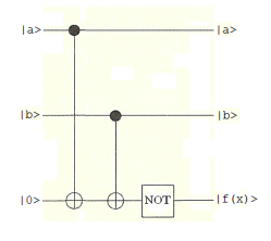
\[ \begin{matrix} \begin{pmatrix} \text{x} & 0 & 1 & 2 & 3 \\ \text{f(x)} & 1 & 0 & 0 & 1 \end{pmatrix} & \text{where} & \begin{matrix} |0 \rangle = |0 \rangle |0 \rangle \\ |1 \rangle = |0 \rangle |1 \rangle \\ |2 \rangle = |1 \rangle |0 \rangle \\ |3 \rangle = |1 \rangle |1 \rangle \end{matrix} \end{matrix} \nonumber \]
The function belongs to the balanced category because it produces 0 and 1 with equal frequency. The modification of this circuit (Deutsch-Jozsa algoritm) highlighted below answers the question of whether the function is constant or balanced (see Julian Brown, The Quest for the Quantum Computer, page 298). Naturally we already know the answer, so this is a simple demonstration that the circuit works.
\[ \begin{matrix} |0 \rangle & \cdots & \fbox{H} & \cdots & \cdot & \cdots & \cdots & \cdots & \cdots & \cdots & \fbox{H} & \triangleright & \text{Measure, 0 or 1} \\ ~ & ~ & ~ & ~ & | \\ |0 \rangle & \cdots & \fbox{H} & \cdots & | & \cdots & \cdot & \cdots & \cdots & \cdots & \fbox{H} & \triangleright & \text{Measure, 0 or 1} \\ ~ & ~ & ~ & ~ & | & ~ & | \\ |1 \rangle & \cdots & \fbox{H} & \cdots & \oplus & \cdots & \oplus & \cdots & \fbox{NOT} & \cdots & \cdots \end{matrix} \nonumber \]
The input is \( |0 \rangle |0 \rangle |1 \rangle : ~ \Psi_{in} = \begin{pmatrix} 0 & 1 & 0 & 0 & 0 & 0 & 0 & 0 \end{pmatrix}^T\)
The following matrices are required to execute the circuit.
\[ \begin{matrix} \text{I} = \begin{pmatrix} 1 & 0 \\ 0 & 1 \end{pmatrix} & \text{NOT} = \begin{pmatrix} 0 & 1 \ 1 & 0 \end{pmatrix} & \text{H} = \frac{1}{ \sqrt{2}} \begin{pmatrix} 1 & 1 \\ 1 & -1 \end{pmatrix} \end{matrix} \nonumber \]
\[ \begin{matrix} \text{CNOT} = \begin{pmatrix} 1 & 0 & 0 & 0 \\ 0 & 1 & 0 & 0 \\ 0 & 0 & 0 & 1 \\ 0 & 0 & 1 & 0 \end{pmatrix} & \text{CnNOT} = \begin{pmatrix} 1 & 0 & 0 & 0 & 0 & 0 & 0 & 0 \\ 0 & 1 & 0 & 0 & 0 & 0 & 0 & 0 \\ 0 & 0 & 1 & 0 & 0 & 0 & 0 & 0 \\ 0 & 0 & 0 & 1 & 0 & 0 & 0 & 0 \\ 0 & 0 & 0 & 0 & 0 & 1 & 0 & 0 \\ 0 & 0 & 0 & 0 & 1 & 0 & 0 & 0 \\ 0 & 0 & 0 & 0 & 0 & 0 & 0 & 1 \\ 0 & 0 & 0 & 0 & 0 & 0 & 1 & 0 \end{pmatrix} \end{matrix} \nonumber \]
The quantum circuit is assembled out of these matrices using tensor (kronecker) multiplication.
\[ \begin{matrix} \text{U}_{ \text{f}} = \text{kronecker(I, kronecker(I, NOT)) kronecker(I, CNOT) CnNOT} \\ \text{QuantumCircuit} = \text{kronecker(H, kronecker(H, I)) U}_{ \text{f}} \text{kronecker(H, kronecker(H, H))} \end{matrix} \nonumber \]
Operation of the quantum circuit on the input vector yields the following result which is written as a product of three qubits on the right.
\[ \begin{matrix} \text{QuantumCircuit} \Psi_{ \text{in}} = \begin{pmatrix} 0 \\ 0 \\ 0 \\ 0 \\ 0 \\ 0 \\ -0.707 \\ 0.707 \end{pmatrix} & \begin{pmatrix} 0 \\ 1 \end{pmatrix} \begin{pmatrix} 0 \\ 1 \end{pmatrix} \frac{1}{ \sqrt{2}} \begin{pmatrix} -1 \\ 1 \end{pmatrix} \end{matrix} \nonumber \]
According to the Deutsch-Jozsa scheme, if both wires are |0> the function is constant, but if at least one wire is |1> the function is balanced. We see by inspection that both wires are |1> indicating that the function is balanced.
The measurements on the top wires can be simulated with projection operators |0><1|, and confirm that the function is not constant but belongs to the balanced category.
\[ \begin{matrix} \text{The first qubit is not |0} \rangle & \left[ \text{kronecker} \left[ \begin{pmatrix} 1 \\ 0 \end{pmatrix} \begin{pmatrix} 1 \\ 0 \end{pmatrix}^T, \text{kronecker(I, I)} \right] \text{QuantumCircuit} \Psi_{ \text{in}} \right]^T = \begin{pmatrix} 0 & 0 & 0 & 0 & 0 & 0 & 0 & 0 \end{pmatrix} \\ \text{The second qubit is not |0} \rangle & \left[ \text{kronecker} \left[ \text{I, kronecker} \left[ \begin{pmatrix} 1 \\ 0 \end{pmatrix} \begin{pmatrix} 1 \\ 0 \end{pmatrix}^T, \text{ I} \right] \right] \text{QuantumCircuit} \Psi_{ \text{in}} \right]^T = \begin{pmatrix} 0 & 0 & 0 & 0 & 0 & 0 & 0 & 0 \end{pmatrix} \\ \text{The first qubit is |1} \rangle & \left[ \text{kronecker} \left[ \begin{pmatrix} 0 \\ 1 \end{pmatrix} \begin{pmatrix} 0 \\ 1 \end{pmatrix}^T, \text{kronecker(I, I)} \right] \text{QuantumCircuit} \Psi_{ \text{in}} \right]^T = \begin{pmatrix} 0 & 0 & 0 & 0 & 0 & 0 & -0.707 & 0.707 \end{pmatrix} \\ \text{The second qubit is |1} \rangle & \left[ \text{kronecker} \left[ \text{I, kronecker} \left[ \begin{pmatrix} 0 \\ 1 \end{pmatrix} \begin{pmatrix} 0 \\ 1 \end{pmatrix}^T, \text{ I} \right] \right] \text{QuantumCircuit} \Psi_{ \text{in}} \right]^T = \begin{pmatrix} 0 & 0 & 0 & 0 & 0 & 0 & -0.707 & 0.707 \end{pmatrix} \end{matrix} \nonumber \]