
8.72: An Illustration of the Deutsch-Jozsa Algorithm
- Page ID
- 148736

The following circuit produces the table of results to its right. The top wires carry the value of x and the circuit places f(x) on the bottom wire. As is shown in the previous tutorial this circuit can also operate in parallel accepting as input all x-values and returning on the bottom wire a superposition of all values of f(x).
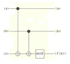
\[ \begin{matrix} \begin{pmatrix} \text{x} & 0 & 1 & 2 & 3 \\ \text{f(x)} & 1 & 0 & 0 & 1 \end{pmatrix} & \text{where} & \begin{matrix} |0 \rangle = |0 \rangle |0 \rangle \\ |1 \rangle = |0 \rangle |1 \rangle \\ |2 \rangle = |1 \rangle |0 \rangle \\ |3 \rangle = |1 \rangle |1 \rangle \end{matrix} \end{matrix} \nonumber \]
The function belongs to the balanced category because it produces 0 and 1 with equal frequency. A modification of this circuit (Deutsch-Jozsa algoritm, p. 298 in The Quest for the Quantum Computer, by Julian Brown) answers the question of whether the function is constant or balanced. Naturally we already know the answer, so this is a simple demonstration that the circuit works.
The input is |0>|0>|1> followed by a Hadamard gate on each wire, as shown in the circuit on page 3. As is well known the Hadamard operation creates the following superposition states.
\[ \begin{matrix} \text{H} \begin{pmatrix} 1 \\ 0 \end{pmatrix} = \frac{1}{ \sqrt{2}} \begin{pmatrix} 1 \\ 1 \end{pmatrix} & \text{H} \begin{pmatrix} 0 \\ 1 \end{pmatrix} = \frac{1}{ \sqrt{2}} \begin{pmatrix} 1 \\ -1 \end{pmatrix} \end{matrix} \nonumber \]
Therefore the Hadamard operation transforms the input state to the following three-qubit state which is fed to the quantum circuit.
\[ \frac{1}{ \sqrt{2}} \begin{pmatrix} 1 \\ 1 \end{pmatrix} \frac{1}{ \sqrt{2}} \begin{pmatrix} 1 \\ 1 \end{pmatrix} \frac{1}{ \sqrt{2}} \begin{pmatrix} 1 \\ -1 \end{pmatrix} = \frac{1}{ 2 \sqrt{2}} \begin{pmatrix} 1 \\ -1 \\ 1 \\ -1 \\ 1 \\ -1 \\ 1 \\ -1 \end{pmatrix} \nonumber \]
The following matrices are required to execute the circuit.
\[ \begin{matrix} \text{I} = \begin{pmatrix} 1 & 0 \\ 0 & 1 \end{pmatrix} & \text{NOT} = \begin{pmatrix} 0 & 1 \\ 1 & 0 \end{pmatrix} & \text{H} = \frac{1}{ \sqrt{2}} \begin{pmatrix} 1 & 1 \\ 1 & -1 \end{pmatrix} \end{matrix} \nonumber \]
\[ \begin{matrix} \text{CNOT} = \begin{pmatrix} 1 & 0 & 0 & 0 \\ 0 & 1 & 0 & 0 \\ 0 & 0 & 0 & 1 \\ 0 & 0 & 1 & 0 \end{pmatrix} & \text{CnNOT} = \begin{pmatrix} 1 & 0 & 0 & 0 & 0 & 0 & 0 & 0 \\ 0 & 1 & 0 & 0 & 0 & 0 & 0 & 0 \\ 0 & 0 & 1 & 0 & 0 & 0 & 0 & 0 \\ 0 & 0 & 0 & 1 & 0 & 0 & 0 & 0 \\ 0 & 0 & 0 & 0 & 0 & 1 & 0 & 0 \\ 0 & 0 & 0 & 0 & 1 & 0 & 0 & 0 \\ 0 & 0 & 0 & 0 & 0 & 0 & 0 & 1 \\ 0 & 0 & 0 & 0 & 0 & 0 & 1 & 0 \end{pmatrix} \end{matrix} \nonumber \]
After the portion of the quantum circuit shown above, Hadamard gates are added to the top two wires, as shown in the circuit on page 3. The matrix representing the circuit is assembled using tensor matrix multiplication and then allowed to operate on the wave function. The full circuit is shown below.
\[ \text{QuantumCircuit} = \text{kronecker(H, kronecker(H, I)) kronecker(I, kronecker(I, NOT)) kronecker(I, CNOT) CnNOT} \nonumber \]
\[ \begin{matrix} \text{QuantumCircuit} = ~ \frac{1}{2} \begin{pmatrix} 0 & 1 & 1 & 0 & 1 & 0 & 0 & 1 \\ 1 & 0 & 0 & 1 & 0 & 1 & 1 & 0 \\ 0 & 1 & -1 & 0 & 1 & 0 & 0 & -1 \\ 1 & 0 & 0 & -1 & 0 & 1 & -1 & 0 \\ 0 & 1 & 1 & 0 & -1 & 0 & 0 & -1 \\ 1 & 0 & 0 & 1 & 0 & -1 & -1 & 0 \\ 0 & 1 & -1 & 0 & -1 & 0 & 0 & 1 \\ 1 & 0 & 0 & -1 & 0 & -1 & 1 & 0 \end{pmatrix} & \text{QuantumCircuit} \frac{1}{2 \sqrt{2}} \begin{pmatrix} 1 \\ -1 \\ 1 \\ -1 \\ 1 \\ -1 \\ 1 \\ -1 \end{pmatrix} = \begin{pmatrix} 0 \\ 0 \\ 0 \\ 0 \\ 0 \\ 0 \\ -0.707 \\ 0.707 \end{pmatrix} & \begin{pmatrix} 0 \\ 1 \end{pmatrix} \begin{pmatrix} 0 \\ 1 \end{pmatrix} \frac{1}{ \sqrt{2}} \begin{pmatrix} -1 \\ 1 \end{pmatrix} \end{matrix} \nonumber \]
Next the qubits on the top two wires are measured. If both are |0> the function is constant, but if at least one is |1> the function is balanced. The measurement on the top wires is implemented with projection operators |0><1|, and confirms that the function is not constant but belongs to the balanced category.
\[ \begin{matrix} \text{The first qubit is not |0} \rangle. & \text{kronecker} \left[ \begin{pmatrix} 1 \\ 0 \end{pmatrix} \begin{pmatrix} 1 \\ 0 \end{pmatrix}^T \text{kronecker(I, I)} \right] \text{QuantumCircuit} \frac{1}{2 \sqrt{2}} \begin{pmatrix} 1 \\ -1 \\ 1 \\ -1 \\ 1 \\ -1 \\ 1 \\ -1 \end{pmatrix} = \begin{pmatrix} 0 \\ 0 \\ 0 \\ 0 \\ 0 \\ 0 \\ 0 \\ 0 \end{pmatrix} \\ \text{The second qubit is not |0} \rangle. & \text{kronecker} \left[ \text{I, kronecker} \left[ \begin{pmatrix} 1 \\ 0 \end{pmatrix} \begin{pmatrix} 1 \\ 0 \end{pmatrix}^T,~ \text{I} \right] \right] \text{QuantumCircuit} \frac{1}{2 \sqrt{2}} \begin{pmatrix} 1 \\ -1 \\ 1 \\ -1 \\ 1 \\ -1 \\ 1 \\ -1 \end{pmatrix} = \begin{pmatrix} 0 \\ 0 \\ 0 \\ 0 \\ 0 \\ 0 \\ 0 \\ 0 \end{pmatrix} \\ \text{The first qubit is |1} \rangle. & \text{kronecker} \left[ \begin{pmatrix} 0 \\ 1 \end{pmatrix} \begin{pmatrix} 0 \\ 1 \end{pmatrix}^T \text{kronecker(I, I)} \right] \text{QuantumCircuit} \frac{1}{2 \sqrt{2}} \begin{pmatrix} 1 \\ -1 \\ 1 \\ -1 \\ 1 \\ -1 \\ 1 \\ -1 \end{pmatrix} = \begin{pmatrix} 0 \\ 0 \\ 0 \\ 0 \\ 0 \\ 0 \\ -0.707 \\ 0.707 \end{pmatrix} \\ \text{The second qubit is |1} \rangle. & \text{kronecker} \left[ \text{I, kronecker} \left[ \begin{pmatrix} 0 \\ 1 \end{pmatrix} \begin{pmatrix} 0 \\ 1 \end{pmatrix}^T, ~ \text{I} \right] \right] \text{QuantumCircuit} \frac{1}{2 \sqrt{2}} \begin{pmatrix} 1 \\ -1 \\ 1 \\ -1 \\ 1 \\ -1 \\ 1 \\ -1 \end{pmatrix} = \begin{pmatrix} 0 \\ 0 \\ 0 \\ 0 \\ 0 \\ 0 \\ -0.707 \\ 0.707 \end{pmatrix} \end{matrix} \nonumber \]
The following illustarted an algebraic analysis of the Deutsch-Jozsa algorithm.
\[ \begin{matrix} \text{Initial} & ~ & 1 & ~ & 2 & ~ & 3 & ~ & 4 & ~ & 5 & ~ & \text{Final} \\ |0 \rangle & \triangleright & \fbox{H} & \cdots & \cdot & \cdots & \cdots & \cdots & \cdots & \cdots & \fbox{H} & \triangleright & \text{Measure, 0 or 1} \\ ~ & ~ & ~ & ~ & | \\ |0 \rangle & \triangleright & \fbox{H} & \cdots & | & \cdots & \cdot & \cdots & \cdots & \cdots & \fbox{H} & \triangleright & \text{Measure, 0 or 1} \\ ~ & ~ & ~ & ~ & | \\ |1 \rangle & \triangleright & \fbox{H} & \cdots & \oplus & \cdots & \oplus & \cdots & \fbox{NOT} & \cdots & \cdots \end{matrix} \nonumber \]
\[ \begin{matrix} \text{H} |0 \rangle \rightarrow \frac{1}{ \sqrt{2}} \left[ |0 \rangle + |1 \rangle \right] & \text{H} |1 \rangle \rightarrow \frac{1}{ \sqrt{2}} \left[ |0 \rangle - |1 \rangle \right] \end{matrix} \nonumber \]
\[ \begin{matrix} \text{NOT} & \text{CNOT} & \text{CnNOT} \\ \begin{pmatrix} 0 & ' & 1 \\ 1 & ' & 0 \end{pmatrix} & \begin{pmatrix} \text{Decimal} & \text{Binary} & ' & \text{Binary} & \text{Decimal} \\ 0 & 00 & ' & 00 & 0 \\ 1 & 01 & ' & 01 & 1 \\ 2 & 10 & ' & 11 & 3 \\ 3 & 11 & ' & 10 & 2 \end{pmatrix} & \begin{pmatrix} \text{Decimal} & \text{Binary} & ' & \text{Binary} & \text{Decimal} \\ 0 & 000 & ' & 000 & 0 \\ 1 & 001 & ' & 001 & 1 \\ 2 & 010 & ' & 010 & 2 \\ 3 & 011 & ' & 011 & 3 \\ 4 & 100 & ' & 101 & 5 \\ 5 & 101 & ' & 100 & 4 \\ 6 & 110 & ' & 111 & 7 \\ 7 & 111 & ' & 110 & 6 \end{pmatrix} \end{matrix} \nonumber \]
\[ \begin{matrix} |000 \rangle \\ \text{H} \otimes \text{H} \otimes \text{H} \\ \frac{1}{ \sqrt{2}} \left[ |0 \rangle + |1 \rangle \right] \frac{1}{ \sqrt{2}} \left[ |0 \rangle + |1 \rangle \right] \frac{1}{ \sqrt{2}} \left[ |0 \rangle - |1 \rangle \right] = \frac{1}{ 2 \sqrt{2}} \left[ |000 \rangle - |001 \rangle + |010 \rangle - |011 \rangle + |100 \rangle - |101 \rangle + |110 \rangle - |111 \rangle \right] \\ \text{CnNOT} \\ \frac{1}{2 \sqrt{2}} \left[ |000 \rangle - |001 \rangle + |010 \rangle - |011 \rangle + |101 \rangle - |100 \rangle + |111 \rangle - |110 \rangle \right] \\ \text{I} \otimes \text{CNOT} \\ \frac{1}{2 \sqrt{2}} \left[ |000 \rangle - |001 \rangle + |011 \rangle - |010 \rangle + |101 \rangle - |100 \rangle + |110 \rangle - |111 \rangle \right] \\ \text{I} \otimes \text{I} \otimes \text{NOT} \\ \frac{1}{ \sqrt{2}} \left[ |0 \rangle - |1 \rangle \right] \frac{1}{ \sqrt{2}} \left[ |0 \rangle - |1 \rangle \right] \frac{1}{ \sqrt{2}} \left[ |1 \rangle - |0 \rangle \right] \\ \text{H} \otimes \text{H} \otimes \text{H} \otimes \text{I} \\ |1 \rangle |1 \rangle \frac{1}{ \sqrt{2}} \left( |1 \rangle - |0 \rangle \right) \end{matrix} \nonumber \]
Since the top wires contain |1 > the function is balanced. This algorithm illustrates the roles of superposition, entanglement and interference in quantum computation. Regarding the latter, it is destructive interference in the last step that eliminates unwanted outcomes yielding the final result on the last line. One pass through the quantum circuit answers the question (is the function balanced or constrant) that would take four calculations on a classical computer.
The interference that occurs in the last step is illustrated by letting |a> = |0> and |b> = |1> and carrying out Hadamard transforms on the first two qubits.
\[ \frac{1}{4 \sqrt{2}} \begin{bmatrix} (a_1 +b_1) (a_2 +b_2)b_3 - (a_1 + b_1)(a_2 +b_2)a_3 \cdots \\ +(a_1 + b_1)(a_2 - b_2) b_3 - (a_1 + b_1)(a_2 - b_2) a_3 \cdots \\ +(a_1 -b_1)(a_2 +b_2)b_3 - (a_1 - b_1)(a_2 + b_2) a_3 \cdots \\ + (a_1 - b_1)(a_2 - b_2) b_3 - (a_1 - b_1)(a_2 -b_2)a_3 \end{bmatrix} ~ \text{simplify} ~ \rightarrow - \frac{ \sqrt{2} a_1 a_2 (a_3 - b_3)}{2} \nonumber \]