8.63: Quantum Correlations Illustrated with Photons

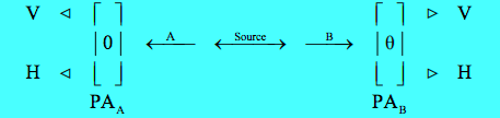
A two-stage atomic cascade emits entangled photons (A and B) in opposite directions with the same circular polarization according to observers in their path. The experiment involves the measurement of photon polarization states in the vertical/horizontal measurement basis, and allows for the rotation of the right-hand detector through an angle θ, in order to explore the consequences of quantum mechanical entanglement. PA stands for polarization analyzer and could simply be a calcite crystal.

The entangled two-photon polarization state is written in the circular and linear polarization bases,

\[ | \Psi \rangle = \frac{1}{ \sqrt{2}} \left[ | L \rangle_A |L \rangle_B + |R \rangle_A |R \rangle_B \right] = \frac{1}{ \sqrt{2}} \left[ |V \rangle_A |V \rangle_B - |H \rangle_A |H \rangle_B \right] \nonumber \]

The vertical (eigenvalue +1) and horizontal (eigenvalue -1) polarization states for the photons in the measurement plane are given below. Θ is the angle of the measuring PA.

\[ \begin{matrix} V( \theta) = \begin{pmatrix} \cos \theta \\ \sin \theta \end{pmatrix} & H( \theta) = \begin{pmatrix} - \sin \theta \\ \cos \theta \end{pmatrix} & V(0) = \begin{pmatrix} 1 \\ 0 \end{pmatrix} & H(0) = \begin{pmatrix} 0 \\ 1 \end{pmatrix} \end{matrix} \nonumber \]

If photon A has vertical polarization photon B also has vertical polarization, the probability that photon B has vertical polarization when measured at an angle θ giving a composite eigenvalue of +1 is,

\[ \left( V( \theta)^T V(0) \right)^2 \rightarrow \cos ( \theta)^2 \nonumber \]

If photon A has vertical polarization photon B also has vertical polarization, the probability that photon B has horizontal polarization when measured at an angle θ giving a composite eigenvalue of -1 is,

\[ \left( H( \theta)^T V(0) \right)^2 \rightarrow \sin ( \theta)^2 \nonumber \]

Therefore the overall quantum correlation coefficient or expectation value is:

\[ E( \theta) = \left( V( \theta)^T V(0) \right)^2 - \left( H( \theta)^T V(0) \right)^2 \text{ simplify } \rightarrow \cos (2 \theta) \nonumber \]

Now it will be shown that a local-realistic, hidden-variable model can be constructed which is in agreement with the quantum calculations for 0, 45 and 90 degrees, but not for 30 and 60 degrees (highlighted).

\[ \begin{matrix} \text{E(0 deg) = 1} & \text{E(30 deg) = 0.5} & \text{E(45 deg) = 0} & \text{E(60 deg) = -0.5} & \text{E(90 deg) = -1} \end{matrix} \nonumber \]

If objects have well-defined properties independent of measurement, the results for θ = 0 degrees and θ = 90 degrees require that the photons carry the following instruction sets, where the hexagonal vertices refer to θ values of 0, 30, 60, 90, 120, and 150 degrees.

There are eight possible instruction sets, six of the type on the left and two of the type on the right. The white circles represent vertical polarization with eigenvalue +1 and the black circles represent horizontal polarization with eigenvalue -1. In any given measurement, according to local realism, both photons (A and B) carry identical instruction sets, in other words the same one of the eight possible sets.

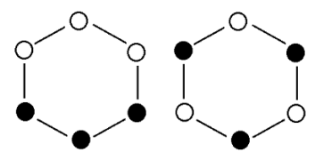
The problem is that while these instruction sets are in agreement with the 0 and 90 degree quantum calculations, with expectation values of +1 and -1 respectively, they can't explain the 30 degree predictions of quantum mechanics. The figure on the left shows that the same result should be obtained 4 times with joint eigenvalue +1, and the opposite result twice with joint eigenvalue of -1. For the figure on the right the opposite polarization is always observed giving a joint eigenvalue of -1. Thus, local realism predicts an expectation value of 0 in disagreement with the quantum result of 0.5.

\[ \frac{6(1-1+1+1-1+1)+2(-1-1-1-1-1-1)}{8} = 0 \nonumber \]

If we look at 60 degrees, E(60 deg) = 0,we reach the same conclusion: local realism disagrees with quantum result of -0.5.

\[ \frac{^(-1-1+1-1-1+1)+2(1+1+1+1+1+1)}{8} = 0 \nonumber \]

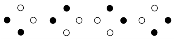
Instruction sets for 45 degrees, E(45 deg) = 0, are shown below. The vertices are 0, 45, 90 and 135 degrees. The instruction sets are constructed so that they satisfy the 0 and 90 degree quantum expectation values of 1 and -1, respectively. It is clear that they also satisfy the 45 degree result yielding an expectation value of zero: (1-1+1-1) = (-1+1-1+1) = (1-1+1-1) = (-1+1-1+1) = 0.

This exercise illustrates Bell's theorem: no local hidden-variable theory can reproduce all the predictions of quantum mechanics for entangled composite systems . As the quantum predictions are confirmed experimentally, the local hidden-variable approach to reality must be abandoned.

This analysis is based on "Simulating Physics with Computers" by Richard Feynman, published in the International Journal of Theoretical Physics (volume 21, pages 481-485), and Julian Brown's Quest for the Quantum Computer (pages 91-100). Feynman used the experiment outlined above to establish that a local classical computer could not simulate quantum physics.

A local classical computer manipulates bits which are in well-defined states, 0s and 1s, shown above graphically in white and black. However, these classical states are incompatible with the quantum mechanical analysis which is consistent with experimental results. This two-photon experiment demonstrates that simulation of quantum physics requires a computer that can manipulate 0s and 1s, superpositions of 0 and 1, and entangled superpositions of 0s and 1s. Simulation of quantum physics requires a quantum computer!