8.53: Bell State Exercises

The Bell states are maximally entangled superpositions of two-particle states. Consider two spin-1/2 particles created in the same event. There are four maximally entangled wave functions representing their collective spin states. Each particle has two possible spin orientations and therefore the composite state is represented by a 4-vector in a four-dimensional Hilbert space.

\[ \begin{matrix} | \Phi_p \rangle = \frac{1}{ \sqrt{2}} \left[ | \uparrow_1 \rangle | \uparrow_2 \rangle + | \downarrow_1 \rangle | \downarrow_2 \rangle \right] = \frac{1}{ \sqrt{2}} \left[ \begin{pmatrix} 1 \\ 0 \end{pmatrix} \otimes \begin{pmatrix} 1 \\ 0 \end{pmatrix} + \begin{pmatrix} 0 \\ 1 \end{pmatrix} \otimes \begin{pmatrix} 0 \\ 1 \end{pmatrix} \right] = \frac{1}{ \sqrt{2}} \begin{pmatrix} 1 \\ 0 \\ 0 \\ 1 \end{pmatrix} & \Phi_p = \frac{1}{ \sqrt{2}} \begin{pmatrix} 1 \\ 0 \\ 0 \\ 1 \end{pmatrix} \\ | \Phi_m \rangle = \frac{1}{ \sqrt{2}} \left[ | \uparrow_1 \rangle | \uparrow_2 \rangle - | \downarrow_1 \rangle | \downarrow_2 \rangle \right] = \frac{1}{ \sqrt{2}} \left[ \begin{pmatrix} 1 \\ 0 \end{pmatrix} \otimes \begin{pmatrix} 1 \\ 0 \end{pmatrix} - \begin{pmatrix} 0 \\ 1 \end{pmatrix} \otimes \begin{pmatrix} 0 \\ 1 \end{pmatrix} \right] = \frac{1}{ \sqrt{2}} \begin{pmatrix} 1 \\ 0 \\ 0 \\ -1 \end{pmatrix} & \Phi_p = \frac{1}{ \sqrt{2}} \begin{pmatrix} 1 \\ 0 \\ 0 \\ -1 \end{pmatrix} \\ | \Psi_p \rangle = \frac{1}{ \sqrt{2}} \left[ | \uparrow_1 \rangle | \downarrow_2 \rangle + | \downarrow_1 \rangle | \uparrow_2 \rangle \right] = \frac{1}{ \sqrt{2}} \left[ \begin{pmatrix} 1 \\ 0 \end{pmatrix} \otimes \begin{pmatrix} 0 \\ 1 \end{pmatrix} + \begin{pmatrix} 0 \\ 1 \end{pmatrix} \otimes \begin{pmatrix} 1 \\ 0 \end{pmatrix} \right] = \frac{1}{ \sqrt{2}} \begin{pmatrix} 0 \\ 1 \\ 1 \\ 0 \end{pmatrix} & \Phi_p = \frac{1}{ \sqrt{2}} \begin{pmatrix} 0 \\ 1 \\ 1 \\ 0 \end{pmatrix} \\ | \Psi_m \rangle = \frac{1}{ \sqrt{2}} \left[ | \uparrow_1 \rangle | \downarrow_2 \rangle - | \downarrow_1 \rangle | \uparrow_2 \rangle \right] = \frac{1}{ \sqrt{2}} \left[ \begin{pmatrix} 1 \\ 0 \end{pmatrix} \otimes \begin{pmatrix} 0 \\ 1 \end{pmatrix} - \begin{pmatrix} 0 \\ 1 \end{pmatrix} \otimes \begin{pmatrix} 1 \\ 0 \end{pmatrix} \right] = \frac{1}{ \sqrt{2}} \begin{pmatrix} 0 \\ 1 \\ -1 \\ 0 \end{pmatrix} & \Phi_p = \frac{1}{ \sqrt{2}} \begin{pmatrix} 0 \\ 1 \\ -1 \\ 0 \end{pmatrix} \end{matrix} \nonumber \]

The wave functions are not separable and consequently the entangled particles represented by these wave functions do not have separate identities or individual properties, they behave like a single entity. Individually the spins don't have a definite polarization, yet there is a definite spin orientation relationship between them. For example, if the spin orientation of particle 1 is learned through measurement, the spin orientation of particle 2 is also immediately known no matter how far away it may be. (The Appendix shows how such measurements destroy entanglement, forcing both particles into well-defined spin states.) Entanglement implies nonlocal phenomena which in the words of Nick Herbert are "unmediated, unmitigated and immediate."

The Bell states can be generated from two classical bits with the use of a quantum circuit involving a Hadamard (H) gate, the identity (I) and a controlled-not gate (CNOT) as shown below. The H gate operates on the top bit creating a superposition which controls the operation of the CNOT gate. The classical state on the left also serves as an index for the Bell state created from it: 0, 1, 2, 3. Kronecker, as discussed below, is Mathcad's command for matrix tensor multiplication.

\[ \begin{matrix} H = \frac{1}{ \sqrt{2}} \begin{pmatrix} 1 & 1 \\ 1 & -1 \end{pmatrix} & I = \begin{pmatrix} 1 & 0 \\ 0 & 1 \end{pmatrix} & \text{CNOT} = \begin{pmatrix} 1 & 0 & 0 & 0 \\ 0 & 1 & 0 & 0 \\ 0 & 0 & 0 & 1 \\ 0 & 0 & 1 & 0 \end{pmatrix} & \begin{matrix} \text{Bell} & | a \rangle & \triangleright & H & \cdot & \triangleright & \text{Bell} \\ \text{State} ~ & ~ & ~ & | & ~ & \beta_{ab} \\ \text{Index} & | \beta \rangle & \triangleright & \cdots & \oplus & \triangleright & \text{State} \end{matrix} \end{matrix} \nonumber \]

Bell state generator:

\[ \text{BSG} = \text{CNOT kronecker(H, I)} \nonumber \]

\[ \begin{matrix} \text{Index = 0} & \text{Index = 1} \\ \begin{pmatrix} 1 \\ 0 \end{pmatrix} \begin{pmatrix} 1 \\ 0 \end{pmatrix} = \begin{pmatrix} 1 \\ 0 \\ 0 \\ 0 \end{pmatrix} ~~ \text{BSG} \begin{pmatrix} 1 \\ 0 \\ 0 \\ 0 \end{pmatrix} = \begin{pmatrix} 0.707 \\ 0 \\ 0 \\ 0.707 \end{pmatrix} & \begin{pmatrix} 1 \\ 0 \end{pmatrix} \begin{pmatrix} 0 \\ 1 \end{pmatrix} = \begin{pmatrix} 0 \\ 1 \\ 0 \\ 0 \end{pmatrix} ~~ \text{BSG} \begin{pmatrix} 0 \\ 1 \\ 0 \\ 0 \end{pmatrix} = \begin{pmatrix} 0 \\ 0.707 \\ 0.707 \\ 0 \end{pmatrix} \\ \text{Index = 2} & \text{Index = 3} \\ \begin{pmatrix} 0 \\ 1 \end{pmatrix} \begin{pmatrix} 1 \\ 0 \end{pmatrix} = \begin{pmatrix} 0 \\ 0 \\ 1 \\ 0 \end{pmatrix} ~~ \text{BSG} \begin{pmatrix} 0 \\ 0 \\ 1 \\ 0 \end{pmatrix} = \begin{pmatrix} 0.707 \\ 0 \\ 0 \\ -0.707 \end{pmatrix} & \begin{pmatrix} 1 \\ 0 \end{pmatrix} \begin{pmatrix} 0 \\ 1 \end{pmatrix} = \begin{pmatrix} 0 \\ 1 \\ 0 \\ 0 \end{pmatrix} ~~ \text{BSG} \begin{pmatrix} 0 \\ 0 \\ 0 \\ 1 \end{pmatrix} = \begin{pmatrix} 0 \\ 0.707 \\ -0.707 \\ 0 \end{pmatrix} \end{matrix} \nonumber \]

It is not surprising that a Bell state measurement (BSM) is just the reverse of this process.

\[ \begin{matrix} \text{Bell} & \triangleright & \cdot & H & \triangleright & | a \rangle & \text{Bell} \\ \beta_{ab} & ~ & | ~ & ~ & ~ & ~ & \text{State} \\ \text{State} & \triangleright & \oplus & \cdots & \triangleright & | b \rangle & \text{Index} \end{matrix} \nonumber \]

\[ \text{BSM = BSG}^{-1} \nonumber \]

\[ \begin{matrix} \text{BSM} \begin{pmatrix} 0.707 \\ 0 \\ 0 \\ 0.707 \end{pmatrix} = \begin{pmatrix} 1 \\ 0 \\ 0 \\ 0 \end{pmatrix} & \text{BSM} \begin{pmatrix} 0 \\ 0.707 \\ 0.707 \\ 0 \end{pmatrix} = \begin{pmatrix} 0 \\ 1 \\ 0 \\ 0 \end{pmatrix} & \text{BSM} \begin{pmatrix} 0.707 \\ 0 \\ 0 \\ -0.707 \end{pmatrix} = \begin{pmatrix} 0 \\ 0 \\ 1 \\ 0 \end{pmatrix} & \text{BSM} \begin{pmatrix} 0 \\ 0.707 \\ -0.707 \\ 0 \end{pmatrix} = \begin{pmatrix} 0 \\ 0 \\ 0 \\ 1 \end{pmatrix} \end{matrix} \nonumber \]

We will now explore some of the characteristics of the Bell states through a variety of calculations. First we list the spin eigenfunctions in the Cartesian directions.

\[ \begin{matrix} \text{Szu} = \begin{pmatrix} 1 \\ 0 \end{pmatrix} & \text{Szd} = \begin{pmatrix} 0 \\ 1 \end{pmatrix} & \text{Sxu} = \frac{1}{ \sqrt{2}} \begin{pmatrix} 1 \\ 1 \end{pmatrix} & \text{Sxd} = \frac{1}{ \sqrt{2}} \begin{pmatrix} -1 \\ 1 \end{pmatrix} & \text{Syu} = \frac{1}{ \sqrt{2}} \begin{pmatrix} 1 \\ i \end{pmatrix} & \text{Syd} = \frac{1}{ \sqrt{2}} \begin{pmatrix} 1 \\ -i \end{pmatrix} \end{matrix} \nonumber \]

Working in units of h/4π we can use the Pauli matrices to represent the spin operators in the Cartesian directions. We will also need the identity operator from above.

\[ \begin{matrix} \sigma_x = \begin{pmatrix} 0 & 1 \\ 1 & 0 \end{pmatrix} & \sigma_y = \begin{pmatrix} 0 & -i \\ i & 0 \end{pmatrix} & \sigma_z = \begin{pmatrix} 1 & 0 \\ 0 & -1 \end{pmatrix} \end{matrix} \nonumber \]

Composite two-particle operators are constructed using matrix tensor multiplication implemented with Mathcad's kronecker command.

\[ \begin{matrix} \text{SxSx} = \text{kroncker}( \sigma_x,~ \sigma_x) & \text{SySy} = \text{kronecker}( \sigma_y,~ \sigma_y) & \text{SzSz} = \text{kroncker} ( \sigma_z,~ \sigma_z) \end{matrix} \nonumber \]

The following matrix demonstrates that the Bell states are an orthonormal basis set.

\[ \begin{pmatrix} \Phi_p^T \Phi_p & \Phi_p^T \Phi_m & \Phi_p^T \Psi_p & \Phi_p^T \Psi_m \\ \Phi_m^T \Phi_p & \Phi_m^T \Phi_m & \Phi_m^T \Psi_p & \Phi_m^T \Psi_m \\ \Psi_p^T \Phi_p & \Psi_p^T \Phi_m & \Psi_p^T \Psi_p & \Psi_p^T \Psi_m \\ \Psi_m^T \Phi_p & \Psi_m^T \Phi_m & \Psi_m^T \Psi_p & \Psi_m^T \Psi_m \\ \end{pmatrix} = \begin{pmatrix} 1 & 0 & 0 & 0 \\ 0 & 1 & 0 & 0 \\ 0 & 0 & 1 & 0 \\ 0 & 0 & 0 & 1 \end{pmatrix} \nonumber \]

In the interest of brevity, the main quantum properties of the Bell states will be illustrated using the spin operator in the z-direction. Calculations involving the x- and y-spin operators can be found in the appendix.

The Bell states are eigenfunctions of the σ_zσ_z, σ_xσ_x and σ_yσ_y spin operators.

\[ \begin{array}{c & c} \text{eigenvalue} = 1 & \text{eigenvalue} = -1 \\ \begin{matrix} SzSz \Phi_p = \begin{pmatrix} 0.707 \\ 0 \\ 0 \\ 0.707 \end{pmatrix} & SzSz \Phi_m = \begin{pmatrix} 0.707 \\ 0 \\ 0 \\ -0.707 \end{pmatrix} \\ SxSx \Phi_p = \begin{pmatrix} 0.707 \\ 0 \\ 0 \\ 0.707 \end{pmatrix} & SxSx \Psi_p = \begin{pmatrix} 0 \\ 0.707 \\ 0.707 \\ 0 \end{pmatrix} \\ SySy \Phi_m = \begin{pmatrix} 0.707 \\ 0 \\ 0 \\ -0.707 \end{pmatrix} & SySy \Psi_p = \begin{pmatrix} 0 \\ 0.707 \\ 0.707 \\ 0 \end{pmatrix} \end{matrix} & \begin{matrix} SzSz \Psi_p = \begin{pmatrix} 0 \\ -0.707 \\ -0.707 \\ 0 \end{pmatrix} & SzSz \Psi_m = \begin{pmatrix} 0 \\ - 0.707 \\ 0.707 \\ 0 \end{pmatrix} \\ SxSx \Phi_m = \begin{pmatrix} - 0.707 \\ 0 \\ 0 \\ 0.707 \end{pmatrix} & SxSx \Psi_m = \begin{pmatrix} 0 \\ -0.707 \\ 0.707 \\ 0 \end{pmatrix} \\ SySy \Phi_p = \begin{pmatrix} -0.707 \\ 0 \\ 0 \\ -0.707 \end{pmatrix} & SySy \Psi_m = \begin{pmatrix} 0 \\ -0.707 \\ 0.707 \\ 0 \end{pmatrix} \end{matrix} \end{array} \nonumber \]

Calculations of the expectation values yield consistent results.

\[ \begin{matrix} \Phi_p^T SzSz \Phi_p = 1 & \Phi_m^T SzSz \Phi_m = 1 & \Psi_p^T SzSz \Psi_p = -1 & \Psi_m^T SzSz \Psi_m = 1 \\ \Phi_p^T SxSx \Phi_p = 1 & \Phi_m^T SxSx \Phi_m = -1 & \Psi_p^T SxSx \Psi_p = 1 & \Psi_m^T SxSx \Psi_m = -1 \\ \Phi_p^T SySy \Phi_p = -1 & \Phi_m^T SySy \Phi_m = 1 & \Psi_p^T SySy \Psi_p = -1 & \Psi_m^T SySy \Psi_m = 1 \\ \end{matrix} \nonumber \]

We see that for the composite measurements in the z-basis the Φ Bell states exhibit perfect correlation, while the Ψ states show perfect anti-correlation. In the x-basis, the p states show perfect correlation and the m states show perfect anti-correlation.

This correlation is striking when you consider that the individual spin measurements on particles 1 and 2 are completely random giving expectation values of zero, as the following calculations show.

\[ \begin{matrix} \Phi_p^T \text{kronecker}( \sigma_z,~I) \Phi_p = 0 & \Phi_p^T \text{kronecker}(I,~ \sigma_z) \Phi_p = 0 \\ \Phi_m^T \text{kronecker}( \sigma_z,~I) \Phi_m = 0 & \Phi_m^T \text{kronecker}(I,~ \sigma_z) \Phi_m = 0 \\ \Psi_p^T \text{kronecker}( \sigma_z,~I) \Phi_p = 0 & \Psi_p^T \text{kronecker}(I,~ \sigma_z) \Psi_p = 0 \\ \Psi_m^T \text{kronecker}( \sigma_z,~I) \Psi_m = 0 & \Psi_m^T \text{kronecker}(I,~ \sigma_z) \Psi_m = 0 \\ \end{matrix} \nonumber \]

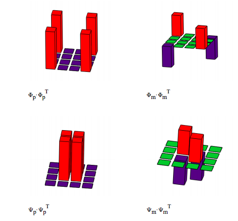
Individually the particles appear to behave like classical mixtures, but collectively they exhibit quantum correlations. We will now look at this issue from another perspective. First the density operators (|Ψ><Ψ|) are calculated for each of the Bell states. (See the Appendix for a graphical representation of the density matrices.

\[ \begin{matrix} \Phi_p \Phi_p^T = \begin{pmatrix} 0.5 & 0 & 0 & 0.5 \\ 0 & 0 & 0 & 0 \\ 0 & 0 & 0 & 0 \\ 0.5 & 0 & 0 & 0.5 \end{pmatrix} & \Phi_m \Phi_m^T = \begin{pmatrix} 0.5 & 0 & 0 & -0.5 \\ 0 & 0 & 0 & 0 \\ 0 & 0 & 0 & 0 \\ -0.5 & 0 & 0 & 0.5 \end{pmatrix} \\ \Psi_p \Psi_p^T = \begin{pmatrix} 0 & 0 & 0 & 0 \\ 0 & 0.5 & 0.5 & 0 \\ 0 & 0.5 & 0.5 & 0 \\ 0 & 0 & 0 & 0 \end{pmatrix} & \Psi_m \Psi_m^T = \begin{pmatrix} 0 & 0 & 0 & 0 \\ 0 & 0.5 & -0.5 & 0 \\ 0 & -0.5 & 0.5 & 0 \\ 0 & 0 & 0 & 0 \end{pmatrix} \end{matrix} \nonumber \]

We also demonstrate that the Bell states are pure states by showing that (|Ψ><Ψ|)² = |Ψ><Ψ|.

\[ \begin{matrix} \left( \Phi_p \Phi_p^T \right)^2 = \begin{pmatrix} 0.5 & 0 & 0 & 0.5 \\ 0 & 0 & 0 & 0 \\ 0 & 0 & 0 & 0 \\ 0.5 & 0 & 0 & 0.5 \end{pmatrix} & \left( \Phi_m \Phi_m^T \right)^2 = \begin{pmatrix} 0.5 & 0 & 0 & -0.5 \\ 0 & 0 & 0 & 0 \\ 0 & 0 & 0 & 0 \\ -0.5 & 0 & 0 & 0.5 \end{pmatrix} \\ \left( \Psi_p \Psi_p^T \right)^2 = \begin{pmatrix} 0 & 0 & 0 & 0 \\ 0 & 0.5 & 0.5 & 0 \\ 0 & 0.5 & 0.5 & 0 \\ 0 & 0 & 0 & 0 \end{pmatrix} & \left( \Psi_m \Psi_m^T \right)^2 = \begin{pmatrix} 0 & 0 & 0 & 0 \\ 0 & 0.5 & -0.5 & 0 \\ 0 & -0.5 & 0.5 & 0 \\ 0 & 0 & 0 & 0 \end{pmatrix} \end{matrix} \nonumber \]

The existence of off-diagonal elements in these matrix operators is the quantum signature of an entangled superposition. We concentrate on the |Φ_m><Φ_m| density operator which is shown below. The following analysis is adapted from AJP 77, 244-252 (2009).

\[ | \Phi_m \rangle \langle \Phi_m | = \frac{1}{2} \left[ | \uparrow_1 \rangle \otimes | \uparrow_2 \rangle - | \downarrow_1 \rangle \otimes | \downarrow_2 \rangle \right] \left[ \langle \uparrow_2 | \otimes \langle \uparrow_1 | - \langle \downarrow_2 | \otimes \langle \downarrow_1 | \right] \nonumber \]

In expanding this expression we will make use of identities like the following, which rearranges 1221 terms as 1122 terms.

\[ | \uparrow_1 \rangle \otimes | \uparrow_2 \rangle \langle \downarrow_2 | \otimes \langle \downarrow_1 | = | \uparrow_1 \rangle \langle \downarrow_1 | \otimes | \uparrow_2 \rangle \langle \downarrow_2 | \nonumber \]

\[ | \Phi_m \rangle \langle \Phi_m | = \frac{1}{2} \left[ | \uparrow_1 \rangle \langle \uparrow_1 | \otimes | \uparrow_2 \rangle \langle \uparrow_2 | - | \uparrow_1 \langle \downarrow_1 | \otimes | \uparrow_2 \rangle \langle \downarrow_2 | - | \downarrow_1 \rangle \langle \uparrow_1 | \otimes | \downarrow_2 \rangle \langle \uparrow_2 | + | \downarrow_1 \rangle \langle \downarrow_1 | \otimes | \downarrow_2 \rangle \langle \downarrow_2 | \right] \nonumber \]

To establish the validity of this arrangement we can recalculate |Φ_m><Φ_m|.

\[ \frac{1}{2} \begin{bmatrix} \text{kronecker} \left[ \begin{pmatrix} 1 \\ 0 \end{pmatrix} \begin{pmatrix} 1 & 0 \end{pmatrix},~ \begin{pmatrix} 1 \\ 0 \end{pmatrix} \begin{pmatrix} 1 & 0 \end{pmatrix} \right] - \text{kronecker} \left[ \begin{pmatrix} 1 \\ 0 \end{pmatrix} \begin{pmatrix} 0 & 1 \end{pmatrix},~ \begin{pmatrix} 1 \\ 0 \end{pmatrix} \begin{pmatrix} 0 & 1 \end{pmatrix} \right] ~ \cdots \\ + \text{-kronecker} \left[ \begin{pmatrix} 0 \\ 1 \end{pmatrix} \begin{pmatrix} 1 & 0 \end{pmatrix},~ \begin{pmatrix} 0 \\ 1 \end{pmatrix} \begin{pmatrix} 1 & 0 \end{pmatrix} \right] + \text{kronecker} \left[ \begin{pmatrix} 0 \\ 1 \end{pmatrix} \begin{pmatrix} 0 & 1 \end{pmatrix},~ \begin{pmatrix} 0 \\ 1 \end{pmatrix} \begin{pmatrix} 0 & 1 \end{pmatrix} \right] \end{bmatrix} = \begin{pmatrix} 0.5 & 0 & 0 & -0.5 \\ 0 & 0 & 0 & 0 \\ 0 & 0 & 0 & 0 \\ -0.5 & 0 & 0 & 0.5 \end{pmatrix} \nonumber \]

The reason for writing |Φ_m><Φ_m| in this form is that it facilitates the calculation of the reduced density operator for particle 1 by "tracing" over the contribution of particle 2, or vice versa. (See the Appendix for a more transparent and thorough presentation of the partial trace.) Here we do the former and see that particle 1's "reduced or local" state operator is diagonal indicating a classical mixed state. This result is consistent with the random behavior observed earlier for the expectation values for the individual particles.

\[ \frac{1}{2} \begin{bmatrix} \begin{pmatrix} 1 \\ 0 \end{pmatrix} \begin{pmatrix} 1 & 0 \end{pmatrix} \text{tr} \left[ \begin{pmatrix} 1 \\ 0 \end{pmatrix} \begin{pmatrix} 1 & 0 \end{pmatrix} \right] - \begin{pmatrix} 1 \\ 0 \end{pmatrix} \begin{pmatrix} 0 & 1 \end{pmatrix} \text{tr} \left[ \begin{pmatrix} 1 \\ 0 \end{pmatrix} \begin{pmatrix} 0 & 1 \end{pmatrix} \right] \cdots \\ + - \left[ \begin{pmatrix} 0 \\ 1 \end{pmatrix} \begin{pmatrix} 1 & 0 \end{pmatrix} \right] \text{tr} \left[ \begin{pmatrix} 0 \\ 1 \end{pmatrix} \begin{pmatrix} 1 & 0 \end{pmatrix} \right] + \begin{pmatrix} 0 \\ 1 \end{pmatrix} \begin{pmatrix} 0 & 1 \end{pmatrix} \text{tr} \left[ \begin{pmatrix} 0 \\ 1 \end{pmatrix} \begin{pmatrix} 0 & 1 \end{pmatrix} \right] \end{bmatrix} = \begin{pmatrix} 0.5 & 0 \\ 0 & 0.5 \end{pmatrix} \nonumber \]

Naturally the same is true if we trace over the contribution of particle 1 to obtain the local state operator of particle 2.

\[ \frac{1}{2} \begin{bmatrix} \text{tr} \left[ \begin{pmatrix} 1 \\ 0 \end{pmatrix} \begin{pmatrix} 1 & 0 \end{pmatrix} \right] \left[ \begin{pmatrix} 1 \\ 0 \end{pmatrix} \begin{pmatrix} 1 & 0 \end{pmatrix} \right] - \text{tr} \left[ \begin{pmatrix} 1 \\ 0 \end{pmatrix} \begin{pmatrix} 0 & 1 \end{pmatrix} \right] \left[ \begin{pmatrix} 1 \\ 0 \end{pmatrix} \begin{pmatrix} 0 & 1 \end{pmatrix} \right] \cdots \\ + - \text{tr} \left[ \begin{pmatrix} 0 \\ 1 \end{pmatrix} \begin{pmatrix} 1 & 0 \end{pmatrix} \right] \left[ \begin{pmatrix} 0 \\ 1 \end{pmatrix} \begin{pmatrix} 1 & 0 \end{pmatrix} \right] + \text{tr} \left[ \begin{pmatrix} 0 \\ 1 \end{pmatrix} \begin{pmatrix} 0 & 1 \end{pmatrix} \right] \left[ \begin{pmatrix} 0 \\ 1 \end{pmatrix} \begin{pmatrix} 0 & 1 \end{pmatrix} \right] \end{bmatrix} = \begin{pmatrix} 0.5 & 0 \\ 0 & 0.5 \end{pmatrix} \nonumber \]

That these local density operators represent mixed states is further demonstrated by showing that for each the trace of the square of density operator is less than 1. The Bell states are pure (see above) because for them the trace of the square of the density operator equals 1.

\[ \begin{matrix} \text{tr} \left[ \begin{pmatrix} 0.5 & 0 \\ 0 & 0.5 \end{pmatrix}^2 \right] = 0.5 & \begin{pmatrix} \text{tr} \left( \Phi_p \Phi_p^T \right)^2 & \text{tr} \left( \Phi_m \Phi_m^T \right)^2 & \text{tr} \left( \Psi_p \Psi_p^T \right)^2 & \text{tr} \left( \Phi_m \Psi_m^T \right)^2 \end{pmatrix} = \begin{pmatrix} 1 & 1 & 1 & 1 \end{pmatrix} \end{matrix} \nonumber \]

These calculations, like the previous ones, also establish that while the composite system is a coherent quantum superposition and pure state, the subsystems of the Bell state, spins 1 and 2, exhibit the classical statistical behavior of mixtures. The quantum correlations of the entangled superposition are only apparent when the measurement results on the individual spins are compared side by side.

Appendix

The following table summarizes the expectation value calculations for all three spin operators.

\[ \begin{pmatrix} \Phi_p^T SxSx \Phi_p & \Phi_p^T SySy \Phi_p & \Phi_p^T SzSz \Phi_p \\ \Phi_m^T SxSx \Phi_m & \Phi_m^T SySy \Phi_m & \Phi_m^T SzSz \Phi_m \\ \Psi_p^T SxSx \Psi_p & \Psi_p^T SySy \Psi_p & \Psi_p^T SzSz \Psi_p \\ \Psi_m^T SxSx \Psi_m & \Psi_m^T SySy \Psi_m & \Psi_m^T SzSz \Psi_m \end{pmatrix} = \begin{pmatrix} 1 & -1 & 1 \\ -1 & 1 & 1 \\ 1 & 1 & -1 \\ -1 & -1 & -1 \end{pmatrix} \nonumber \]

This calculation can also be performed by tracing over the product of the density operator and the appropriate spin operator.

\[ \langle \Psi | \hat{A} | \Psi \rangle = \sum_a \langle \Psi | \hat{A} | a \rangle \langle a | \Psi \rangle = \sum_a \langle a | \Psi \rangle \langle \Psi | \hat{A} | a \rangle = Tr \left( | \Psi \rangle \langle \Psi | \hat{A} \right) \nonumber \]

\[ \begin{pmatrix} \text{tr} \left( \Phi_p \Phi_p^T SxSx \right) & \text{tr} \left( \Phi_p \Phi_p^T SySy \right) & \text{tr} \left( \Phi_p \Phi_p^T SzSz \right) \\ \text{tr} \left( \Phi_m \Phi_m^T SxSx \right) & \text{tr} \left( \Phi_m \Phi_m^T SySy \right) & \text{tr} \left( \Phi_m \Phi_m^T SzSz \right) \\ \text{tr} \left( \Psi_p \Psi_p^T SxSx \right) & \text{tr} \left( \Psi_p \Psi_p^T SySy \right) & \text{tr} \left( \Psi_p \Psi_p^T SzSz \right) \\ \text{tr} \left( \Psi_m \Psi_m^T SxSx \right) & \text{tr} \left( \Psi_m \Psi_m^T SySy \right) & \text{tr} \left( \Psi_m \Psi_m^T SzSz \right) \end{pmatrix} = \begin{pmatrix} 1 & -1 & 1 \\ -1 & 1 & 1 \\ 1 & 1 & -1 \\ -1 & -1 & -1 \end{pmatrix} \nonumber \]

It is clear from these results that the Bell states are eigenvectors of the total spin-spin operator.

\[ \begin{matrix} H = \text{kronecker} \left( \sigma_x,~ \sigma_x \right) + \text{kronecker} \left( \sigma_y,~ \sigma_y \right) + \text{kronecker} \left( \sigma_z,~ \sigma_z \right) & H = \begin{pmatrix} 1 & 0 & 0 & 0 \\ 0 & -1 & 2 & 0 \\ 0 & 2 & -1 & 0 \\ 0 & 0 & 0 & 1 \end{pmatrix} \end{matrix} \nonumber \]

\[ \begin{matrix} \Psi_m^T H \Psi_m = -3 & \Psi_p^T H \Psi_p = 1 & \Phi_p^T H \Phi_p = 1 & \Phi_m^T H \Phi_m = 1 \end{matrix} \nonumber \]

\[ -3 \Psi_m \Psi_m^T + \Psi_p \Psi_p^T + \Phi_p \Phi_p^T + \Phi_m \Phi_m^T = \begin{pmatrix} 1 & 0 & 0 & 0 \\ 0 & -1 & 2 & 0 \\ 0 & 2 & -1 & 0 \\ 0 & 0 & 0 & 1 \end{pmatrix} \nonumber \]

More about the partial trace:

The partial trace as given above is not particularly transparent in its matrix implementation. Here the partial trace over spin 1 is presented using conventional Dirac notation. First |Φ_m><Φ_m| is expanded.

\[ | \Phi_m \rangle \langle \Phi_m | = \frac{1}{2} \left[ | \uparrow_1 \rangle | \uparrow_2 \rangle \langle \uparrow_2 | \langle \uparrow_1 | - | \uparrow_1 \rangle | \uparrow_2 \rangle \langle \downarrow_2 | \langle \downarrow_1 | - | \downarrow_1 \rangle | \downarrow_2 \rangle \langle \uparrow_2 | \langle \uparrow_1 | + | \downarrow_1 \rangle | \downarrow_2 \rangle \langle \downarrow_2 | \downarrow_1 | \right] \nonumber \]

Now the trace of spin 1 (bue) is generated showing that the cross terms in the middle of the above expression (red) vanish leaving the following result.

\[ \frac{1}{2} \left[ \langle \uparrow_1 | \Phi_m \rangle \langle \Phi_m | \uparrow_1 \rangle + \langle \downarrow_1 | \Phi_m \rangle \langle \Phi_m | \downarrow_1 \rangle \right] = \frac{1}{2} \left[ | \uparrow_2 \rangle \langle \uparrow_2 | + | \downarrow_2 \rangle \langle \downarrow_2 | \right] \nonumber \]

Wave function collapse:

Previously it was noted that if the spin orientation of particle 1 is learned through measurement, the spin orientation of particle 2 is also immediately known no matter how far away it may be. To show this we first create projection (measurement) operators for spin up and down in the z- and x-directions.

\[ \begin{matrix} P_{zu} = \begin{pmatrix} 1 \\ 0 \end{pmatrix} \begin{pmatrix} 1 & 0 \end{pmatrix} \rightarrow \begin{pmatrix} 1 & 0 \\ 0 & 0 \end{pmatrix} & P_{zd} = \begin{pmatrix} 0 \\ 1 \end{pmatrix} \begin{pmatrix} 0 & 1 \end{pmatrix} \rightarrow \begin{pmatrix} 0 & 0 \\ 0 & 1 \end{pmatrix} \\ P_{zu} = \begin{pmatrix} \frac{1}{ \sqrt{2}} \\ \frac{1}{ \sqrt{2}} \end{pmatrix} \begin{pmatrix} \frac{1}{ \sqrt{2}} & \frac{1}{ \sqrt{2}} \end{pmatrix} \rightarrow \begin{pmatrix} \frac{1}{2} & \frac{1}{2} \\ \frac{1}{2} & \frac{1}{2} \end{pmatrix} & P_{zd} = \begin{pmatrix} \frac{1}{ \sqrt{2}} \\ - \frac{1}{ \sqrt{2}} \end{pmatrix} \begin{pmatrix} \frac{1}{ \sqrt{2}} & - \frac{1}{ \sqrt{2}} \end{pmatrix} \rightarrow \begin{pmatrix} \frac{1}{2} & - \frac{1}{2} \\ - \frac{1}{2} & \frac{1}{2} \end{pmatrix} \end{matrix} \nonumber \]

For the Bell state Ψ_p, measurement of the z-direction spin of the first particle has two equally likely (probability 1/2) outcomes - spin-up or spin-down. These measurement outcomes cause the second particle to have the opposite spin. This result can, of course, be easily predicted by inspection of Ψ_p.

\[ \Psi_p = \frac{1}{ \sqrt{2}} \left[ \begin{pmatrix} 1 \\ 0 \end{pmatrix} \begin{pmatrix} 0 \\ 1 \end{pmatrix} + \begin{pmatrix} 0 \\ 1 \end{pmatrix} \begin{pmatrix} 1 \\ 0 \end{pmatrix} \right] ~~ \begin{matrix} \text{kronecker}(P_{zu},~ I) \Psi_p = \begin{pmatrix} 0 \\ 0.707 \\ 0 \\ 0 \end{pmatrix} & \frac{1}{ \sqrt{2}} \begin{pmatrix} 1 \\ 0 \end{pmatrix} \begin{pmatrix} 0 \\ 1 \end{pmatrix} \\ \text{kronecker}(P_{zd},~ I) \Psi_p = \begin{pmatrix} 0 \\ 0 \\ 0.707 \\ 0 \end{pmatrix} & \frac{1}{ \sqrt{2}} \begin{pmatrix} 0 \\ 1 \end{pmatrix} \begin{pmatrix} 1 \\ 0 \end{pmatrix} \end{matrix} \nonumber \]

Measurement of the x-direction spin of the first particle has two equally likely (probability 1/2) outcomes - spin-up or spin-down. However, for Ψ_p the measurements cause the second particle to have the same spin. This result is not obtained by inspection because the Bell states have been written in the z-basis.

\[ \begin{matrix} \text{kronecker}(P_{xu},~I) \Psi_p = \begin{pmatrix} 0.354 & 0.354 & 0.354 & 0.354 \end{pmatrix} & \frac{1}{ \sqrt{2}} \frac{1}{ \sqrt{2}} \begin{pmatrix} 1 \\ 1 \end{pmatrix} \frac{1}{ \sqrt{2}} \begin{pmatrix} 1 \\ 1 \end{pmatrix} \\ \text{kronecker}(P_{xd},~I) \Psi_p = \begin{pmatrix} -0.354 & 0.354 & 0.354 & -0.354 \end{pmatrix} & \frac{-1}{ \sqrt{2}} \frac{1}{ \sqrt{2}} \begin{pmatrix} 1 \\ -1 \end{pmatrix} \frac{1}{ \sqrt{2}} \begin{pmatrix} 1 \\ -1 \end{pmatrix} \end{matrix} \nonumber \]

This seemingly peculiar result occurs because in the x-basis Ψ_p has the following form.

\[ \Psi_p = \frac{1}{ \sqrt{2}} \left[ \frac{1}{ \sqrt{2}} \begin{pmatrix} 1 \\ 1 \end{pmatrix} \frac{1}{ \sqrt{2}} \begin{pmatrix} 1 \\ 1 \end{pmatrix} - \frac{1}{ \sqrt{2}} \begin{pmatrix} 1 \\ -1 \end{pmatrix} \frac{1}{ \sqrt{2}} \begin{pmatrix} 1 \\ -1 \end{pmatrix} \right] = \frac{1}{ \sqrt{2}} \begin{pmatrix} 0 \\ 1 \\ 1 \\ 0 \end{pmatrix} \nonumber \]

Naturally, these results are consistent with the following expectation values.

\[ \begin{matrix} \Psi_p^T SzSz \Psi_p = -1 & \Psi_p^T SxSx \Psi_p = 1 \end{matrix} \nonumber \]

If we repeat these calculations using Φ_m the following results are obtained.

\[ \Psi_p = \frac{1}{ \sqrt{2}} \left[ \begin{pmatrix} 1 \\ 0 \end{pmatrix} \begin{pmatrix} 1 \\ 0 \end{pmatrix} - \begin{pmatrix} 0 \\ 1 \end{pmatrix} \begin{pmatrix} 0 \\ 1 \end{pmatrix} \right] ~~ \begin{matrix} \text{kronecker}(P_{zu},~ I) \Phi_m = \begin{pmatrix} 0.707 \\ 0 \\ 0 \\ 0 \end{pmatrix} & \frac{1}{ \sqrt{2}} \begin{pmatrix} 1 \\ 0 \end{pmatrix} \begin{pmatrix} 1 \\ 0 \end{pmatrix} \\ \text{kronecker}(P_{zd},~ I) \Phi_m = \begin{pmatrix} 0 \\ 0 \\ 0 \\ -0.707 \end{pmatrix} & \frac{-1}{ \sqrt{2}} \begin{pmatrix} 0 \\ 1 \end{pmatrix} \begin{pmatrix} 0 \\ 1 \end{pmatrix} \end{matrix} \nonumber \]

The z-direction measurements can again be predicted by simple inspection of the entangled wave function.

\[ \begin{matrix} \text{kronecker}(P_{xu},~I) \Phi_m = \begin{pmatrix} 0.354 & -0.354 & 0.354 & -0.354 \end{pmatrix} & \frac{1}{ \sqrt{2}} \frac{1}{ \sqrt{2}} \begin{pmatrix} 1 \\ 1 \end{pmatrix} \frac{1}{ \sqrt{2}} \begin{pmatrix} 1 \\ -1 \end{pmatrix} \\ \text{kronecker}(P_{xd},~I) \Phi_m = \begin{pmatrix} 0.354 & 0.354 & -0.354 & -0.354 \end{pmatrix} & \frac{-1}{ \sqrt{2}} \frac{1}{ \sqrt{2}} \begin{pmatrix} 1 \\ -1 \end{pmatrix} \frac{1}{ \sqrt{2}} \begin{pmatrix} 1 \\ 1 \end{pmatrix} \end{matrix} \nonumber \]

The x-direction results are obvious if we write Φ_m in the x-basis.

\[ \Phi_m = \frac{1}{ \sqrt{2}} \left[ \frac{1}{ \sqrt{2}} \begin{pmatrix} 1 \\ 1 \end{pmatrix} \frac{1}{ \sqrt{2}} \begin{pmatrix} 1 \\ -1 \end{pmatrix} + \frac{1}{ \sqrt{2}} \begin{pmatrix} 1 \\ -1 \end{pmatrix} \frac{1}{ \sqrt{2}} \begin{pmatrix} 1 \\ 1 \end{pmatrix} \right] = \frac{1}{ \sqrt{2}} \begin{pmatrix} 1 \\ 0 \\ 0 \\ -1 \end{pmatrix} \nonumber \]

The results are also consisten with the appropriate expectation values.

\[ \begin{matrix} \Phi_m^T SzSz \Phi_m = 1 & \Phi_m^T SxSx \Phi_m = -1 \end{matrix} \nonumber \]

Graphical representations of the Bell state density matrices:

Algebraic analysis of Bell state generation (read left to right) and Bell state measurement (read right to left).

\[ \begin{matrix} \begin{pmatrix} 1 \\ 0 \\ 0 \\ 0 \end{pmatrix} = | 0 \rangle | 0 \rangle \underleftrightarrow{H \otimes I} \frac{1}{ \sqrt{2}} ( | 0 \rangle + | 1 \rangle) | 0 \rangle = \frac{1}{ \sqrt{2}} (|00 \rangle + | 10 \rangle) \underleftrightarrow{CNOT} \frac{1}{ \sqrt{2}} ( | 00 \rangle + |11 \rangle ) = \frac{1}{ \sqrt{2}} \begin{pmatrix} 1 \\ 0 \\ 0 \\ 1 \end{pmatrix} \\ \begin{pmatrix} 0 \\ 1 \\ 0 \\ 0 \end{pmatrix} = | 0 \rangle | 1 \rangle \underleftrightarrow{H \otimes I} \frac{1}{ \sqrt{2}} ( | 0 \rangle + | 1 \rangle) | 1 \rangle = \frac{1}{ \sqrt{2}} (|01 \rangle + | 11 \rangle) \underleftrightarrow{CNOT} \frac{1}{ \sqrt{2}} ( | 01 \rangle + |10 \rangle ) = \frac{1}{ \sqrt{2}} \begin{pmatrix} 0 \\ 1 \\ 1 \\ 0 \end{pmatrix} \\ \begin{pmatrix} 0 \\ 0 \\ 1 \\ 0 \end{pmatrix} = | 1 \rangle | 0 \rangle \underleftrightarrow{H \otimes I} \frac{1}{ \sqrt{2}} ( | 0 \rangle - | 1 \rangle) | 0 \rangle = \frac{1}{ \sqrt{2}} (|00 \rangle - | 10 \rangle) \underleftrightarrow{CNOT} \frac{1}{ \sqrt{2}} ( | 00 \rangle - |11 \rangle ) = \frac{1}{ \sqrt{2}} \begin{pmatrix} 1 \\ 0 \\ 0 \\ -1 \end{pmatrix} \\ \begin{pmatrix} 0 \\ 0 \\ 0 \\ 1 \end{pmatrix} = | 1 \rangle | 01\rangle \underleftrightarrow{H \otimes I} \frac{1}{ \sqrt{2}} ( | 0 \rangle - | 1 \rangle) | 1 \rangle = \frac{1}{ \sqrt{2}} (|01 \rangle - | 11 \rangle) \underleftrightarrow{CNOT} \frac{1}{ \sqrt{2}} ( | 00 \rangle + |11 \rangle ) = \frac{1}{ \sqrt{2}} \begin{pmatrix} 0 \\ 1 \\ -1 \\ 0 \end{pmatrix} \end{matrix} \nonumber \]