8.49: EPR Analysis for a Composite Singlet Spin System

A spin-1/2 pair is prepared in an entangled singlet state and the individual particles travel in opposite directions on the y-axis to a pair of Stern-Gerlach detectors which are set up to measure spin in the x-z plane. Particle 1's spin is measured along the z-axis, and particle 2's spin is measured at an angle θ with respect to the z-axis.

For the singlet state the arrows below indicate the spin orientation for any direction in the x-z plane.

\[ | \Psi \rangle = \frac{1}{ \sqrt{2}} \left[ | \uparrow \rangle_1 | \downarrow \rangle_2 - | \downarrow \rangle_1 | \uparrow \rangle_2 \right] = \frac{1}{ \sqrt{2}} \left[ \begin{pmatrix} \cos \left( \frac{ \theta}{2} \right) \\ \sin \left( \frac{ \theta}{2} \right) \end{pmatrix}_1 \otimes \begin{pmatrix} - \sin \left( \frac{ \theta}{2} \right) \\ \cos \left( \frac{ \theta}{2} \right) \end{pmatrix}_2 - \begin{pmatrix} - \sin \left( \frac{ \theta}{2} \right) \\ \cos \left( \frac{ \theta}{2} \right) \end{pmatrix}_1 \otimes \begin{pmatrix} \cos \left( \frac{ \theta}{2} \right) \\ \sin \left( \frac{ \theta}{2} \right) \end{pmatrix}_2 \right] = \frac{1}{ \sqrt{2}} \begin{pmatrix} 0 \\ 1 \\ -1 \\ 0 \end{pmatrix} \nonumber \]

The single particle spin operator in the x-z plane is constructed from the Pauli spin operators in the xand z-directions. θ is the angle of orientation of the measurement magnet with the z-axis.

\[ \begin{matrix} \sigma_z = \begin{pmatrix} 1 & 0 \\ 0 & -1 \end{pmatrix} & \sigma_x = \begin{pmatrix} 0 & 1 \\ 1 & 0 \end{pmatrix} & \sigma ( \theta) = \cos ( \theta) \sigma_z + \sin ( \theta) \sigma_x \rightarrow \begin{pmatrix} \cos ( \theta) & \sin ( \theta) \\ \sin ( \theta) & - \cos ( \theta) \end{pmatrix} \end{matrix} \nonumber \]

Tensor multiplication of σ_z and σ(θ) creates a joint spin measurement operator.

\[ \begin{pmatrix} 1 & 0 \\ 0 & -1 \end{pmatrix} \otimes \begin{pmatrix} \cos \theta & \sin \theta \\ \sin \theta & - \cos \theta \end{pmatrix} = \begin{pmatrix} \cos \theta & \sin \theta & 0 & 0 \\ \sin \theta & - \cos \theta & 0 & 0 \\ 0 & 0 & - \cos \theta & - \sin \theta \\ 0 & 0 & - \sin \theta & \cos \theta \end{pmatrix} \nonumber \]

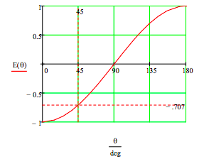
The expectation value as a function of the measurement angle of particle 2 is calculated and the result is displayed graphically.

\[ E( \theta) = \frac{1}{ \sqrt{2}} \begin{pmatrix} 0 & 1 & -1 & 0 \end{pmatrix} \begin{pmatrix} \cos \theta & \sin \theta & 0 & 0 \\ \sin \theta & - \cos \theta & 0 & 0 \\ 0 & 0 & - \cos \theta & - \sin \theta \\ 0 & 0 & - \sin \theta & \cos \theta \end{pmatrix} \frac{1}{ \sqrt{2}} \begin{pmatrix} 0 \\ 1 \\ -1 \\ 0 \end{pmatrix} \rightarrow - \cos \theta \nonumber \]

The expectation value measures correlation. For θ = 0⁰ there is perfect anti-correlation; for θ = 180⁰ perfect correlation (see the Appendix for a discussion of this case); for θ = 900 no correlation; for θ = 45⁰ intermediate anti-correlation (-0.707). Calculations provided in the Appendix show that the individual spin measurements on particles 1 and 2 are totally random for all values of θ, i.e. E(θ) = 0.

\[ \begin{matrix} E \text{(0 deg)} = -1 & E \text{(180 deg)} = 1 & E \text{(90 deg)} = 0 & E \text{(45 deg)} = -0.707 \end{matrix} \nonumber \]

If both observers measure their spins in the z-direction quantum mechanics predicts they will get opposite values due to the singlet nature of the spin state. In other words, the combined expectation value is -1 for these measurements. If spin 2 is measured in the x-direction (θ = 90^o) quantum mechanics predicts, as noted above, an expectation value of 0.

A realist believes that objects have well-defined properties prior to and independent of observation. The following table provide a local realist's explanation of these results. Specific z- and x-spin states are assigned to the particles in the first two columns, with each particle in one of four equally probable spin orientations consistent with the composite singlet state.

\[ \begin{bmatrix} \text{Particle 1} & \text{Particle 2} & \hat{ \sigma}_z (1) \hat{ \sigma}_z (2) & \hat{ \sigma}_z (1) \hat{ \sigma}_x (2) \\ | \uparrow_z \rangle | \uparrow_x \rangle & | \downarrow_z \rangle | \downarrow_x \rangle & -1 & -1 \\ | \uparrow_z \rangle | \downarrow_x \rangle & | \downarrow_z \rangle | \uparrow_x \rangle & -1 & 1 \\ | \downarrow_z \rangle | \uparrow_x \rangle & | \uparrow_z \rangle | \downarrow_x \rangle & -1 & 1 \\ | \downarrow_z \rangle | \downarrow_x \rangle & | \uparrow_z \rangle | \uparrow_x \rangle & -1 & -1 \\ \text{Expectation} & \text{Value} & -1 & 0 \end{bmatrix} \nonumber \]

The quantum and classical pictures agree on the prediction of experimental results. The difficulty is that quantum mechanics does not accept the legitimacy of the states shown in the table on the left. One way to state the problem is to note that σ_x and σ_z are noncommuting operators.

\[ \sigma_z \sigma_x - \sigma_x \sigma_z \rightarrow \begin{pmatrix} 0 & 2 \\ -2 & 0 \end{pmatrix} \nonumber \]

According to quantum mechanics spin in the z- and x-directions cannot simultaneously have well-defined values. The states in the table are not valid, in spite of their agreement with experimental results, because they give well-defined values to incompatible observables. Of course, the realist counters that these arguments simply indicate that quantum mechanics is not a complete theory because it cannot assign definite values to all elements of reality prior to and independent of measurement.

If the second spin is measured in the diagonal direction, θ = 45^o, the realist again predicts an expectation value of 0, as shown in the following table.

\[ \begin{bmatrix} \text{Particle 1} & \text{Particle 2} & \hat{ \sigma}_z (1) \hat{ \sigma}_d (2) \\ | \uparrow_z \rangle | \uparrow_d \rangle & | \downarrow_z \rangle | \downarrow_d \rangle & -1 \\ | \uparrow_z \rangle | \downarrow_d \rangle & | \downarrow_z \rangle | \uparrow_d \rangle & 1 \\ | \downarrow_z \rangle | \uparrow_d \rangle & | \uparrow_z \rangle | \downarrow_d \rangle & 1 \\ | \downarrow_z \rangle | \downarrow_d \rangle & | \uparrow_z \rangle | \uparrow_d \rangle & -1 \\ \text{Expectation} & \text{Value} & 0 \end{bmatrix} \nonumber \]

The spin states in this table are also invalid according to quantum theory.

\[ \sigma_z \sigma \left( \frac{ \pi}{4} \right) - \sigma \left( \frac{ \pi}{4} \right) \sigma_z \rightarrow \begin{pmatrix} 0 & \sqrt{2} \\ - \sqrt{2} & 0 \end{pmatrix} \nonumber \]

However, as calculated earlier quantum mechanics predicts an expectation value of -0.707. This example illustrates Bell's theorem: no local realist hidden-variable theory can reproduce all the predictions of quantum mechanics for entangled composite systems. As the quantum predictions are confirmed experimentally, the local hidden-variable approach to reality must be abandoned. Appendix If particle 2's detector is rotated by 180 degrees, spin-up in the z-direction (blue in the table below) has eigenvalue -1 and spin-down (red in the table below) has eigenvalue +1.

\[ \begin{matrix} \sigma \text{(180 deg)} = \begin{pmatrix} -1 & 0 \\ 0 & 1 \end{pmatrix} & \text{eigenvec}( \sigma \text{(180 deg), -1)} = \begin{pmatrix} 1 \\ 0 \end{pmatrix} & \text{eigenvec} ( \sigma \text{(180 deg), 1)} = \begin{pmatrix} 0 \\ 1 \end{pmatrix} \end{matrix} \nonumber \]

This leads to the local realist predictions in the right-hand column, which are in agreement with quantum mechanics.

\[ \begin{bmatrix} \text{Particle 1} & \text{Particle 2} & \hat{ \sigma}_z (1) \hat{ \sigma}_z ^{ \pi} (2) \\ | \uparrow_z \rangle | \uparrow_x \rangle & | \downarrow_z \rangle | \downarrow_x \rangle & 1 \\ | \uparrow_z \rangle | \downarrow_x \rangle & | \downarrow_z \rangle | \uparrow_x \rangle & 1 \\ | \downarrow_z \rangle | \uparrow_x \rangle & | \uparrow_z \rangle | \downarrow_x \rangle & 1 \\ | \downarrow_z \rangle | \downarrow_x \rangle & | \uparrow_z \rangle | \uparrow_x \rangle & 1 \\ \text{Expectation} & \text{Value} & 1 \end{bmatrix} \nonumber \]

The following operator is used to calculate the expectation value for measurements on spin 2 as a function of the detector angle θ. The identity operator represents no measurement on spin 1.

\[ \begin{pmatrix} 1 & 0 \\ 0 & 1 \end{pmatrix} \otimes \begin{pmatrix} \cos \theta & \sin \theta \\ \sin \theta & - \cos \theta \end{pmatrix} = \begin{pmatrix} \cos \theta & \sin \theta & 0 & 0 \\ \sin \theta & - \cos \theta & 0 & 0 \\ 0 & 0 & \cos \theta & \sin \theta \\ 0 & 0 & \sin \theta & - \cos \theta \end{pmatrix} \nonumber \]

The following calculation shows that the measurement results are totally random, yielding and an expectation value of 0 for all values of θ.

\[ E ( \theta) = \frac{1}{ \sqrt{2}} \begin{pmatrix} 0 & 1 & -1 & 0 \end{pmatrix} \begin{pmatrix} \cos \theta & \sin \theta & 0 & 0 \\ \sin \theta & - \cos \theta & 0 & 0 \\ 0 & 0 & \cos \theta & \sin \theta \\ 0 & 0 & \sin \theta & - \cos \theta \end{pmatrix} \frac{1}{ \sqrt{2}} \begin{pmatrix} 0 \\ 1 \\ -1 \\ 0 \end{pmatrix} \rightarrow 0 \nonumber \]

The same, of course, is true for the measurements on spin 1.

\[ \begin{pmatrix} \cos \theta & \sin \theta \\ \sin \theta & - \cos \theta \end{pmatrix} \otimes \begin{pmatrix} 1 & 0 \\ 0 & 1 \end{pmatrix} = \begin{pmatrix} \cos \theta & 0 & \sin \theta & 0 \\ 0 & \cos \theta & 0 & \sin \theta \\ \sin \theta & 0 & - \cos \theta & 0 \\ 0 & \sin \theta & 0 & - \cos \theta \end{pmatrix} \nonumber \]

\[ E ( \theta) = \frac{1}{ \sqrt{2}} \begin{pmatrix} 0 & 1 & -1 & 0 \end{pmatrix} \begin{pmatrix} \cos \theta & 0 & \sin \theta & 0 \\ 0 & \cos \theta & 0 & \sin \theta \\ \sin \theta & 0 & - \cos \theta & 0 \\ 0 & \sin \theta & 0 & - \cos \theta \end{pmatrix} \frac{1}{ \sqrt{2}} \begin{pmatrix} 0 \\ 1 \\ -1 \\ 0 \end{pmatrix} \rightarrow 0 \nonumber \]

The expectation value calculations can also be performed using the trace function as shown below.

\[ \langle \Psi | \hat{O} | \Psi \rangle = \sum_i \langle \Psi | \hat{O} | i \rangle \langle i | \Psi \rangle = \sum_i \langle i | \Psi \rangle \langle \Psi | \hat{O} | i \rangle = Trace \left( | \Psi \rangle \langle \Psi | \hat{O} \right) ~ \text{where} ~ \sum_i |i \rangle \langle i | = \text{Identity} \nonumber \]