8.40: Another GHZ Example Using Spin-1/2 Particles

Last updated
Save as PDF

Page ID: 144050

\( \newcommand{\vecs}[1]{\overset { \scriptstyle \rightharpoonup} {\mathbf{#1}} } \) \( \newcommand{\vecd}[1]{\overset{-\!-\!\rightharpoonup}{\vphantom{a}\smash {#1}}} \)\(\newcommand{\id}{\mathrm{id}}\) \( \newcommand{\Span}{\mathrm{span}}\) \( \newcommand{\kernel}{\mathrm{null}\,}\) \( \newcommand{\range}{\mathrm{range}\,}\) \( \newcommand{\RealPart}{\mathrm{Re}}\) \( \newcommand{\ImaginaryPart}{\mathrm{Im}}\) \( \newcommand{\Argument}{\mathrm{Arg}}\) \( \newcommand{\norm}[1]{\| #1 \|}\) \( \newcommand{\inner}[2]{\langle #1, #2 \rangle}\) \( \newcommand{\Span}{\mathrm{span}}\) \(\newcommand{\id}{\mathrm{id}}\) \( \newcommand{\Span}{\mathrm{span}}\) \( \newcommand{\kernel}{\mathrm{null}\,}\) \( \newcommand{\range}{\mathrm{range}\,}\) \( \newcommand{\RealPart}{\mathrm{Re}}\) \( \newcommand{\ImaginaryPart}{\mathrm{Im}}\) \( \newcommand{\Argument}{\mathrm{Arg}}\) \( \newcommand{\norm}[1]{\| #1 \|}\) \( \newcommand{\inner}[2]{\langle #1, #2 \rangle}\) \( \newcommand{\Span}{\mathrm{span}}\)\(\newcommand{\AA}{\unicode[.8,0]{x212B}}\)

This exercise explores the outcomes of measurements on the three spin-1/2 entangled state, Ψ_ABC, highlighted below. It represents a lean GHZ protocol developed by H. J. Bernstein. Because much has been published on the GHZ protocol, I'm going to get right to the point without a lot of commentary.

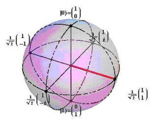
The eigenstates for spin-up and spin-down in the z-, x- and y-directions in vector format are as follows.

\[ \begin{matrix} Z_u = \begin{pmatrix} 1 \\ 0 \end{pmatrix} & Z_d = \begin{pmatrix} 0 \\ 1 \end{pmatrix} & X_u = \frac{1}{ \sqrt{2}} \begin{pmatrix} 1 \\ 1 \end{pmatrix} & X_d = \frac{1}{ \sqrt{2}} \begin{pmatrix} 1 \\ -1 \end{pmatrix} & Y_u = \frac{1}{ \sqrt{2}} \begin{pmatrix} 1 \\ i \end{pmatrix} & Y_d = \frac{1}{ \sqrt{2}} \begin{pmatrix} 1 \\ -i \end{pmatrix} \end{matrix} \nonumber \]

These spin states are also shown on a Bloch sphere.

Screen Shot 2019-03-29 at 1.50.28 PM.png

Tensor multiplication using Mathcad commands will be used to form the initial entangled spin state and subsequent measurement states. These results can be easily verified by hand calculation.

\[ \Psi \text{(a, b, c)} = \text{submatrix} \left[ \text{kronecker} \left[ \text{augment} \left[ \text{a, } \begin{pmatrix} 0 \\ 0 \end{pmatrix} \right], ~ \text{kronecker} \left[ \text{augment} \left[ \text{b, } \begin{pmatrix} 0 \\ 0 \end{pmatrix} \right], ~ \text{augment} \left[ \text{c, } \begin{pmatrix} 0 \\ 0 \end{pmatrix} \right] \right] \right], 1,~8,~1,~1 \right] \nonumber \]

Initial state:

\[ \begin{matrix} \Psi_{ABC} = \frac{1}{ \sqrt{2}} \left( \Psi \left( Y_u,~Y_u,~Y_u \right) - \Psi \left( Y_d,~Y_d,~Y_d \right) \right) & \Psi_{ABC}^T = \begin{pmatrix} 0 & 0.5i & 0.5i & 0 & 0.5i 0 & 0 & -0.5i \end{pmatrix} \end{matrix} \nonumber \]

Given this initial state the probabilities for the various measurement outcomes for spin in the z-direction are calculated.

\[ \begin{matrix} \left( \left| \Psi (Z_u,~ Z_u,~ Z_u)^T \Psi_{ABC} \right| \right)^2 = 0 & \left( \left| \Psi (Z_u,~ Z_u,~ Z_d)^T \Psi_{ABC} \right| \right)^2 = 0.25 & \left( \left| \Psi (Z_u, ~Z_d, ~Z_u)^T \Psi_{ABC} \right| \right)^2 = 0.25 \\ \left( \left| \Psi (Z_d,~ Z_u, ~Z_u)^T \Psi_{ABC} \right| \right)^2 = 0.25 & \left( \left| \Psi (Z_u,~ Z_d,~ Z_d)^T \Psi_{ABC} \right| \right)^2 = 0 & \left( \left| \Psi (Z_d,~ Z_u,~ Z_d)^T \Psi_{ABC} \right| \right)^2 = 0 \\ \left( \left| \Psi (Z_d,~ Z_d,~ Z_u)^T \Psi_{ABC} \right| \right)^2 = 0 & \left( \left| \Psi (Z_d,~ Z_d,~ Z_d)^T \Psi_{ABC} \right| \right)^2 = 0.25 \end{matrix} \nonumber \]

These calculations predict that the following spin states are observed: Z_uZ_uZ_d, Z_uZ_dZ_u, Z_dZ_uZ_u and Z_dZ_dZ_d. It is easily seen that the measurement of any two spin-states allows the prediction of the third without the need for a measurement. If two spins have the same value (uu or dd) then the third is d. If two spin states have different values (ud or du) then the third is u. Einstein, Podolsky and Rosen (EPR) wrote in their famous 1935 Physical Review paper,

"If, without in any way disturbing a system, we can predict with certainty (i.e. with probability equal to unity) the value of a physical quantity, then there exists an element of reality corresponding to this physical quantity."

According to this definition spin in the z-direction is an "element of reality." In other words, it has a definite value independent of measurement.

Next we calculate the quantum mechanical predictions for the measurement of spin in the x-direction on two of the spins and in the z-direction for the third.

\[ \begin{matrix} \left( \left| \Psi (Z_u,~X_u~Z_u)^T \Psi_{ABC} \right| \right)^2 = 0 & \left( \left| \Psi (X_u,~X_u,~Z_d) ^T \Psi_{ABC} \right| \right)^2 = 0.25 & \left( \left| \Psi (X_u, X_d,~ X_u)^T \Psi_{ABC} \right| \right)^2 = 0.25 \\ \left( \left| \Psi (X_u,~ X_d,~ Z_d)^T \Psi_{ABC} \right| \right)^2 = 0.25 & \left( \left| \Psi (X_d,~X_u,~Z_u)^T \Psi_{ABC} \right| \right)^2 = 0 & \left( \left| \Psi (X_d,~ X_u,~ Z_d)^T \Psi_{ABC} \right| \right)^2 = 0 \\ \left( \left| \Psi (X_d,~ X_d,~ Z_d)^T \Psi_{ABC} \right| \right)^2 = 0 & \left( \left| \Psi (X_d,~ X_d,~ Z_u)^T \Psi_{ABC} \right| \right)^2 = 0.25 \\ \left( \left| \Psi (X_u,~ Z_u,~ X_u)^T \Psi_{ABC} \right| \right)^2 = 0 & \left( \left| \Psi (X_u,~ Z_d, X_u)^T \Psi_{ABC} \right| \right)^2 = 0.25 & \left( \left| \Psi (X_u,~ Z_u,~ X_d)^T \Psi_{ABC} \right| \right)^2 = 0.25 \\ \left( \left| \Psi (X_u,~ Z_d,~ X_d)^T \Psi_{ABC} \right| \right)^2 = 0.25 & \left( \left| \Psi (X_d,~ Z_u,~ X_u)^T \Psi_{ABC} \right| \right)^2 = 0 & \left( \left| \Psi (X_d,~ Z_d,~ X_u)^T \Psi_{ABC} \right| \right)^2 = 0 \\ \left( \left| \Psi (X_u,~ Z_d,~ X_d)^T \Psi_{ABC} \right| \right)^2 = 0 & \left( \left| \Psi (X_d,~ Z_u,~ X_d)^T \Psi_{ABC} \right| \right)^2 = 0.25 \\ \left( \left| \Psi (Z_u,~ X_u,~X_u)^T \Psi_{ABC} \right| \right)^2 = 0 & \left( \left| \Psi (Z_d,~X_u,~X_u)^T \Psi_{ABC} \right| \right)^2 = 0.25 & \left( \left| \Psi (Z_u, X_u, X_d)^T \Psi_{ABC} \right| \right)^2 = 0.25 \\ \left( \left| \Psi (Z_d,~X_u,~X_d)^T \Psi_{ABC} \right| \right)^2 = 0.25 & \left( \left| \Psi (Z_u, X_d, X_u)^T \Psi_{ABC} \right| \right)^2 = 0 & \left( \left| \Psi (Z_d,~X_d,~X_u)^T \Psi_{ABC} \right| \right)^2 = 0 \\ \left( \left| \Psi (Z_d,~X_d,~X_d)^T \Psi_{ABC} \right| \right)^2 = 0 & \left( \left| \Psi (Z_u,~X_d,~X_d)^T \Psi_{ABC} \right| \right)^2 = 0.25 \end{matrix} \nonumber \]

The twelve possible outcomes are listed in two rows.

\[ \begin{pmatrix} X_uX_uZ_u & X_dX_dZ_u & X_uZ_uX_u & X_dZ_uX_d & Z_uX_uX_u & Z_uX_dX_d \\ X_dX_dZ_d & X_dX_uZ_d & X_uZ_dX_d & X_dZ_dX_u & Z_dX_uX_d & Z_dX_dX_u \end{pmatrix} \nonumber \]

These results are summarized as follows: if two spins have the same x-spin state then the z-spin state is u, but if they are different the z-spin state is d. Again according to the EPR criterion spin in the z-direction is an element of reality.

However, the calculations can be described in another way: (a) measurements in which three pairs have the same x spin state and (b) measurements in which one pair has the same x-spin state and the remaining pairs have different x-spin states. The following table organizes the experimental results grouped in these categories. The first two rows satisfy criterion (a) and the remaining six rows satisfy criterion (b). The left column shows the implied total x-spin state, the middle three columns how it is achieved, and the right column the z-spin state consistent with the x-spin measurement results.

\[ \begin{pmatrix} X_uX_uX_u & ' & X_uX_uZ_d & Z_uX_uX_u & X_uZ_uX_u & ' & Z_uZ_uZ_u \\ X_dX_dX_d & ' & X_dX_dZ_u & X_dZ_uX_d & Z_uX_dX_d & ' & Z_uZ_uZ_u \\ X_uX_uX_d & ' & X_uX_uZ_u & X_uZ_dX_d & Z_dX_uX_d & ' & Z_dZ_dZ_u \\ X_dX_dX_u & ' & X_dX_dZ_u & X_dZ_dX_u & Z_dX_dX_u & ' & Z_dZ_dZ_u \\ X_uX_dX_u & ' & X_uZ_uX_u & X_uX_dZ_d & Z_dX_dX_u & ' & Z_dZ_uZ_d \\ X_dX_uX_d & ' & X_dZ_uX_d & X_dX_uZ_d & Z_dX_uX_d & ' & Z_dZ_uZ_d \\ X_dX_uX_u & ' & Z_uX_uX_u & X_dZ_dX_u & X_dX_uZ_d & ' & Z_uZ_dZ_d \\ X_uX_dX_d & ' & Z_uX_dX_d & X_uZ_dX_d & X_uX_dZ_d & ' & Z_uZ_dZ_d \end{pmatrix} \nonumber \]

As this table demonstrates, according to the x-direction spin measurements the permissible z-direction states are Z_uZ_uZ_u, Z_dZ_dZ_u, Z_dZ_uZ_d and Z_uZ_dZ_d. This is in direct contradiction to the earlier z-direction measurements which gave the result Z_dZ_dZ_d, Z_uZ_uZ_d, Z_uZ_dZ_u and Z_dZ_dZ_u, using the same initial wavefunction Ψ_ABC. In other words two measurement protocols lead to the notion that z-direction spin is an element of reality according to the EPR definition, but they dramatically disagree on the actual z-direction spin values allowed.

In the February 2001 issue of the American Journal of Physics on page 187, John D. Norton summarizes the situation as follows:

Two principal assumptions were made in the arguments that generated this contradiction. One was that the empirical predictions of quantum theory are reliable. The other was the EPR reality criterion, which in turn, depends on the assumptions of separability and locality. One of these assumptions must be given up. The continuing empirical success of quantum theory has led to a consensus that it is the second assumption, the EPR reality criterion, which is to be discarded.