8.39: A GHZ Gedanken Experiment Using Spatial Degrees of Freedom and Tensor Algebra

Tensor algebra is used to simplify the mathematical analysis of a gedanken experiment presented by John D. Norton in the February 2011 issue of the American Journal of Physics (pp 182-188). Norton's construction using spatial degrees of freedom is in my opinion highly contrived and actually not as simple as the original GHZ experiment involving polarized light [Nature 404, 515-519 (2000)] or Mermin's gedanken rendition involving spin-1/2 particles [Physics Today 43(6), 9-11 (1990)]. Besides using tensor algebra to avoid tedious algebraic manipulations, I adopt a more plausible model for the two-chambered Einstein boxes employed in Norton's approach.

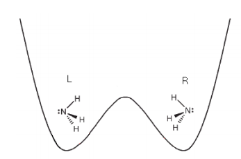
The thought experiment involves three widely separated two-chamber boxes which I prefer to model as infinite potential wells with a finite internal barrier, as shown below. What I have in mind here is a simplified model for the ammonia molecule. See the Appendix for a more realistic double-well potential.

The orthonormal vectors |L> and |R> given below represent occupancy in the two chambers. Norton initially considers the consequences of placing the particle in two states, |P> and |M>, which are also orthonormal. I have no idea how these states would be created, and this is the main reason I find Norton's approach artificial.

\[ \begin{matrix} L = \begin{pmatrix} 1 \\ 0 \end{pmatrix} & R = \begin{pmatrix} 0 \\ 1 \end{pmatrix} & L^T L = 1 & R^T R = 1 & L^T = 0 \\ P = \frac{1}{ \sqrt{2}} (L + iR) & M = \frac{1}{ \sqrt{2}} (L - iR) & \overline{(P^T)}P = 1 & \overline{(M^T)} M = 1 & \overline{(P^T)}M = 0 \end{matrix} \nonumber \]

In the second part of my analysis I use the following symmetric and anti-symmetric states. These represent the ground and first excited superposition states of the ammonia molecule regarding the position of the nitrogen atom to the left or right of the plane created by the three hydrogen atoms.

\[ \begin{matrix} S = \frac{1}{ \sqrt{2}} (L+R) & A = \frac{1}{ \sqrt{2}} (L-R) & S^T S = 1 & A^T A = 1 & A^T S = 0 \end{matrix} \nonumber \]

Construction of the initial three-box state highlighted below is facilitated by the use of three Mathcad commands: submatrix, kronecker, and augment. It is not difficult to do this by hand, however having a general expression for the wavefunction simplifies subsequent analysis.

\[ \Psi \text{a, b, c} = \text{submatrix} \left[ \text{kronecker} \left[ \text{augment} \left[ a, \begin{pmatrix} 0 \\ 0 \end{pmatrix} \right],~ \text{kronecker} \left[ \text{augment} \left[ b,~ \begin{pmatrix} 0 \\ 0 \end{pmatrix} \right], ~ \text{augment} \left[ c,~ \begin{pmatrix} 0 \\ 0 \end{pmatrix} \right] \right] \right],~ 1,~ 8,~ 1,~ 1 \right] \nonumber \]

Initial state:

\[ \begin{matrix} \Psi_{ABC} = \frac{1}{ \sqrt{2}} ( \Psi \text{ (P, P, P)} - \Psi \text{M, M, M))} & \Psi_{ABC}^T = \begin{pmatrix} 0 & 0.5i & 0.5i & 0 & 0.5i & 0 & 0 & -0.5i \end{pmatrix} \end{matrix} \nonumber \]

For a three-box system this initial entangled states has eight possible position measurement outcomes, four of which are observed as shown in the probability calculations below.

\[ \begin{matrix} \left( \left| \Psi \text{(L, L, L)}^T \Psi_{ABC} \right| \right)^2 = 0 & \left( \left| \Psi \text{(L, L, R)}^T \Psi_{ABC} \right| \right)^2 = 0.25 & \left( \left| \Psi \text{(L, R, L)}^T \Psi_{ABC} \right| \right)^2 = 0.25 \\ \left( \left| \Psi \text{(R, L, L)}^T \Psi_{ABC} \right| \right)^2 = 0.25 & \left( \left| \Psi \text{(L, R, R)}^T \Psi_{ABC} \right| \right)^2 = 0 & \left( \left| \Psi \text{(R, L, R)}^T \Psi_{ABC} \right| \right)^2 = 0 \\ \left( \left| \Psi \text{(R, R, L)}^T \Psi_{ABC} \right| \right)^2 = 0 & \left( \left| \Psi \text{(R, R, R)}^T \Psi_{ABC} \right| \right)^2 = 0.25 \end{matrix} \nonumber \]

These results show that position measurements on any two of the boxes enables one to determine which chamber the particle occupies in the third box without further measurement. If the measured particles are found to be on the same side (either both L or both R) the third particle is in the right chamber R. If they are different, the third particle is in the left chamber, L. Because we can predict with certainty the position of the particle in the third box, we say its position is an "element of reality." This leads to the conclusion that the permissible position eigenstates are: LLR, LRL, RLL, and RRR.

In a second set of experiments we shine light on two of the boxes with a frequency that just matches the energy difference between the ground state |S> and excited state |A>. If the light is absorbed the box is in the |S> state; if the box is in the |A> state stimulated emission occurs and a photon is released. This set of experiments measures the spectroscopic states of the boxes.

As the following probability calculations show, if the two boxes irradiated are found to be in the same spectroscopic state (SS or AA) a subsequent measurement of the position of the particle in the third box will yield L. Conversely, if they are in different spectroscopic state the position measurement on the third box will yield R. Thus, this set of measurements also indicate that position is an "element of reality."

\[ \begin{matrix} \left( \left| \Psi \text{(S, S, L)}^T \Psi_{ABC} \right| \right)^2 = 0 & \left( \left| \Psi \text{(S, S, R)}^T \Psi_{ABC} \right| \right)^2 = 0.25 & \left( \left| \Psi \text{(S, A, L)}^T \Psi_{ABC} \right| \right)^2 = 0.25 \\ \left( \left| \Psi \text{(S, A, R)}^T \Psi_{ABC} \right| \right)^2 = 0.25 & \left( \left| \Psi \text{(A, S, L)}^T \Psi_{ABC} \right| \right)^2 = 0 & \left( \left| \Psi \text{(A, S, R)}^T \Psi_{ABC} \right| \right)^2 = 0 \\ \left( \left| \Psi \text{(A, A, R)}^T \Psi_{ABC} \right| \right)^2 = 0 & \left( \left| \Psi \text{(A, A, L)}^T \Psi_{ABC} \right| \right)^2 = 0.25 \\ \left( \left| \Psi \text{(S, L, S)}^T \Psi_{ABC} \right| \right)^2 = 0 & \left( \left| \Psi \text{(S, R, S)}^T \Psi_{ABC} \right| \right)^2 = 0.25 & \left( \left| \Psi \text{(S, L, A)}^T \Psi_{ABC} \right| \right)^2 = 0.25 \\ \left( \left| \Psi \text{(S, R, A)}^T \Psi_{ABC} \right| \right)^2 = 0.25 & \left( \left| \Psi \text{(A, L, S)}^T \Psi_{ABC} \right| \right)^2 = 0 & \left( \left| \Psi \text{(A, R, S)}^T \Psi_{ABC} \right| \right)^2 = 0 \\ \left( \left| \Psi \text{(A, R, A)}^T \Psi_{ABC} \right| \right)^2 = 0 & \left( \left| \Psi \text{(A, L, A)}^T \Psi_{ABC} \right| \right)^2 = 0.25 \\ \left( \left| \Psi \text{(L, S, S)}^T \Psi_{ABC} \right| \right)^2 = 0 & \left( \left| \Psi \text{(R, S, S)}^T \Psi_{ABC} \right| \right)^2 = 0.25 & \left( \left| \Psi \text{(L, S, A)}^T \Psi_{ABC} \right| \right)^2 = 0.25 \\ \left( \left| \Psi \text{(R, S, A)}^T \Psi_{ABC} \right| \right)^2 = 0.25 & \left( \left| \Psi \text{(L, A, S)}^T \Psi_{ABC} \right| \right)^2 = 0 & \left( \left| \Psi \text{(R, A, S)}^T \Psi_{ABC} \right| \right)^2 = 0 \\ \left( \left| \Psi \text{(R, A, A)}^T \Psi_{ABC} \right| \right)^2 = 0 & \left( \left| \Psi \text{(L, A, A)}^T \Psi_{ABC} \right| \right)^2 = 0.25 \end{matrix} \nonumber \]

The allowed states for these measurements are listed in the following table. The top row showing that SS or AA implies L and that SA or AS implies R.

\[ \begin{pmatrix} \text{SSL} & \text{AAL} & \text{SLS} & \text{ALA} & \text{LSS} & \text{LAA} \\ \text{SAR} & \text{ASR} & \text{SRA} & \text{ARS} & \text{RSA} & \text{RAS} \end{pmatrix} \nonumber \]

The measurement outcomes can also be grouped in two different ways: (a) measurements in which three pairs have the same spectroscopic state and (b) measurements in which one pair has the same spectroscopic state and the remaining pairs have different spectroscopic states. The following table organizes the experimental results grouped in these categories. The first two rows satisfy criterion (a) and the remaining six rows satisfy criterion (b). The left column shows the implied total spectroscopic state, the middle three columns how it is achieved, and the right column the position state consistent with the spectroscopic results.

\[ \begin{pmatrix} \text{SSS} & ' & \text{SSL} & \text{LSS} & \text{SLS} & ' & \text{LLL} \\ \text{AAA} & ' & \text{AAL} & \text{ALA} & \text{LAA} & ' & \text{LLL} \\ \text{SSA} & ' & \text{SSL} & \text{SRA} & \text{RSA} & ' & \text{RRL} \\ \text{AAS} & ' & \text{AAL} & \text{ARS} & \text{RAS} & ' & \text{RRL} \\ \text{SAS} & ' & \text{SLS} & \text{SAR} & \text{RAS} & ' & \text{RLR} \\ \text{ASA} & ' & \text{ALA} & \text{ASR} & \text{RSA} & ' & \text{RLR} \\ \text{ASS} & ' & \text{LSS} & \text{ARS} & \text{ASR} & ' & \text{LRR} \\ \text{SAA} & ' & \text{LAA} & \text{SRA} & \text{SAR} & ' & \text{LRR} \end{pmatrix} \nonumber \]

As this table demonstrates, according to the spectroscopic measurements the permissible position states are RRL, RLR, LRR and LLL. This is in direct contradiction to the earlier position measurements which gave the result LLR, LRL, RLL, and RRR. In other words two measurement protocols lead to the notion that position is an element of reality, but they dramatically disagree on the actual values of the allowed positions. Norton concludes his paper with the following assessment.

Two principal assumptions were made in the arguments that generated this contradiction. One was that the empirical predictions of quantum theory are reliable. The other was that the EPR reality criterion, which in turn, depends on the assumptions of separability and locality. One of these assumptions must be given up. The continuing empirical success of quantum theory has led to a consensus that it is the second assumption, the EPR reality criterion, which is to be discarded.

Appendix

A more realistic potential well for this problem is shown below.