8.16: GHZ Entanglement - A Tensor Algebra Analysis

This tutorial analyses experimental results on a GHZ entanglement reported by Anton Zeilinger and collaborators in the 3 February 2000 issue of Nature (pp. 515‐519) using tensor algebra. The GHZ experiment employs three‐photon entanglement to provide a stunning attack on local realism.

First some definitions:

• Realism ‐ experiments yield values for properties that exist independent of experimental observation
• Locality ‐ the experimental results obtained at location A at time t, do not depend on the results at some other location B at time t.
• H/V = horizontal/vertical linear polarization.
• R/L = right/left circular polarization. Hʹ/Vʹ rotated by 45^o with respect to H/V.

Next the vector representations of the various photon polarization states:

\[ \begin{matrix} H = \begin{pmatrix} 1 \\ 0 \end{pmatrix} & V = \begin{pmatrix} 0 \\ 1 \end{pmatrix} & H' = \frac{1}{ \sqrt{2}} \begin{pmatrix} 1 \\ 1 \end{pmatrix} & V' = \frac{1}{ \sqrt{2}} \begin{pmatrix} 1 \\ -1 \end{pmatrix} & L = \frac{1}{ \sqrt{2}} \begin{pmatrix} 1 \\ -i \end{pmatrix} & R = \frac{1}{ \sqrt{2}} \begin{pmatrix} 1 \\ i \end{pmatrix} & N = \begin{pmatrix} 0 \\ 0 \end{pmatrix} \end{matrix} \nonumber \]

Some additional matrices needed to form state vectors in Mathcad:

\[ \begin{matrix} \text{HN = augment (H, N)} & \text{VN = augment (V, N)} & \text{RN = augment (R, N)} \\ \text{LN = augment (L, N)} & \text{H'N = augment (H', N)} & \text{V'N = augment (V', N)} \end{matrix} \nonumber \]

The operators associated with linear and cicular polarization:

\[ \begin{matrix} H'V = \begin{pmatrix} 0 & 1 \\ 1 & 0 \end{pmatrix} & RL = \begin{pmatrix} 0 & -1 \\ i & 0 \end{pmatrix} \end{matrix} \nonumber \]

The initial GHZ three-phon entangled state:

\[ \Psi = \frac{1}{ \sqrt{2}} (H_1 H_2 H_3 + V_1 V_2 V_3) \nonumber \]

Initial state expressed in tensor format:

\[ | \Psi \rangle = \frac{1}{ \sqrt{2}} \left[ \begin{pmatrix} 1 \\ 0 \end{pmatrix} \otimes \begin{pmatrix} 1 \\ 0 \end{pmatrix} \otimes \begin{pmatrix} 1 \\ 0 \end{pmatrix} + \begin{pmatrix} 0 \\ 1 \end{pmatrix} \otimes \begin{pmatrix} 0 \\ 1 \end{pmatrix} \otimes \begin{pmatrix} 0 \\ 1 \end{pmatrix} \right] = \frac{1}{ \sqrt{2}} \begin{pmatrix} 1 \\ 0 \\ 0 \\ 0 \\ 0 \\ 0 \\ 0 \\ 1 \end{pmatrix} \nonumber \]

Constructing the initial state using Mathcad:

\[ \Psi = \frac{1}{ \sqrt{2}} \text{submatrix}(\text{kronecker (HN, HN)}) + \text{kronecker( VN, kronecker (VN, VN))}, 1,~8,~1,~1) \nonumber \]

\[ \Psi^T = \begin{pmatrix} 0 & 0 & 0 & 0 & 0 & 0 & 0.707 \end{pmatrix} \nonumber \]

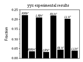
After preparation of the initial GHZ state (see figure 1 in the reference cited above), polarization measurements are performed on the three photons. Zeilinger and collaborators use y to stand for a circular polarization measurement and x for a linear polarization measurement. Initially they perform circular polarization measurements on two of the photons and a linear polarization measurement on the other photon. The quantum mechanically predicted results and actual experimental measurements are given below.

yyx - experiment

The yyx operator is calculated and it is shown that Ψ is an eigenstate of the operator with eigenvalue ‐1.

\[ \begin{matrix} \text{yyx} = \text{kronecker(RL, kronecker(RL, H'V'))} & \Psi^T \text{yyx} \Psi = -1 \end{matrix} \nonumber \]

Each measurement (R/L or Hʹ/Vʹ) has two possible outcomes so, in principle, there could be 8 possible results. However, quantum mechanics predicts that only four equally probable outcomes are possible. This is because the eigenvalues of the individual results must be consistent with the eigenvalue the total operator. As shown below, the eigenvalues for Hʹ and R are +1, and for Vʹ and L they are ‐1.

\[ \begin{matrix} H'V'H' = \begin{pmatrix} 0.707 \\ 0.707 \end{pmatrix} & H'V'V' = \begin{pmatrix} -0.707 \\ 0.707 \end{pmatrix} & RLR = \begin{pmatrix} 0.707 \\ 0.707i \end{pmatrix} & RLL = \begin{pmatrix} -0.707 \\ 0.707i \end{pmatrix} \end{matrix} \nonumber \]

Thus quantum mechanics predicts that RRVʹ (++‐), LRHʹ (‐++), RLHʹ (+‐+), and LLVʹ (‐‐‐) should be observed, but RRHʹ (+++), LRVʹ (‐+‐), RLVʹ (+‐‐) and LLHʹ (‐‐+) should not be observed. This prediction is in agreement with the experimental results shown in Figure 1 to within experimental error.

Figure 1.

Confirm the first two results in figure 1.

\[ \begin{matrix} RRV' = \text{submatrix(kronecker(RN, kronecker(RN, V'N))},~ 1,~8,~1,~1) (|RRV' \Psi |)^2 = 0.25 \\ RRH' = \text{submatrix(kronecker(RN, kronecker(RN, H'N))},~ 1,~8,~1,~1) (|RRH' \Psi |)^2 = 0 \end{matrix} \nonumber \]

For the two remaining experiments in this class (yxy and xyy), the agreement between theoretical prediction and experimental results is basically the same.

While these agreements between quantum mechanics and experiment are impressive they do not directly challenge the local realist position. As will be shown later that will be accomplished by a fourth experiment involving the measurement of the linear polarization on all three photons ‐ the xxx experiment.

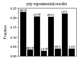
yxy - experiment

The yxy operator is calculated and it is shown that Ψ is an eigenstate of the operator with eigenvalue -1.

\[ \begin{matrix} \text{yxy} = \text{kronecker(RL, kronecker(H'V', RL))} & \Psi^T yxy \Psi = -1 \end{matrix} \nonumber \]

Using reasoning identical to the yyx experiment, quantum mechanics predicts that RVʹR (+‐+), LHʹR (‐++), RHʹL (++‐), and LVʹL (‐‐‐) should be observed, but RHʹR (+++), LVʹR (‐‐+), RVʹL (+‐‐) and LHʹL (‐+‐) should not be observed. This prediction is in agreement with the experimental results shown in Figure 2 to within experimental error.

Figure 2.

Confirm the first two results in Figure 2.

\[ \begin{matrix} RV'R = \text{submatrix(kronecker(RN, kronecker(V'N, RN))},~ 1,~8,~1,~1) \\ (|RV'R \Psi |)^2 = 0.25 \\ RH'R = \text{submatrix(kronecker(RN, kronecker(H'N, RN))},~ 1,~8,~1,~1) \\ (|RH'R \Psi |)^2 = 0 \end{matrix} \nonumber \]

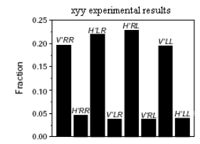
xyy - experiment

The xyy operator is calculated and it is shown that Ψ is an eigenstate of the operator with eigenvalue ‐1.

\[ \begin{matrix} \text{xyy} = \text{kronecker(H'V', kronecker(RL, RL))} & \Psi^T \text{xyy} \Psi = -1 \end{matrix} \nonumber \]

Using reasoning identical to the previous experiments, quantum mechanics predicts that VʹRR (‐++), HʹLR (+‐+), HʹRL (++‐), and VʹLL (‐‐‐) should be observed, but HʹRR (+++), VʹLR (‐‐+), VʹRL (‐+‐) and HʹLL (+‐‐) should not be observed. This prediction is in agreement with the experimental results shown in Figure 3 to within experimental error.

Figure 3.

Confirm the first two results in Figure 3.

\[ \begin{matrix} \text{V'RR} = \text{submatrix(kronecker(V'N, kronecker(RN RN))},~ 1,~ 8,~ 1,~ 1) (|V'RR \Psi |)^2 = 0.25 \\ \text{H'RR} = \text{submatrix(kronecker(H'N, kronecker(RN, RN))},~ 1,~ 8,~ 1,~ 1) (| H'RR \Psi |)^2 = 0 \end{matrix} \nonumber \]

Now for the critical experiment.

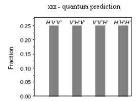
xxx - experiment

The xxx operator is calculated and it is shown that Ψ is an eigenstate of the operator with eigenvalue +1.

\[ \begin{matrix} \text{xxx} = \text{kronecker(H'V', kronecker(H'V', H'V'))} & \Psi^T \text{xxx} \Psi = 1 \end{matrix} \nonumber \]

Using reasoning identical to the previous experiments, quantum mechanics predicts that only HʹVʹVʹ (+‐‐), VʹHʹVʹ (‐+‐), VʹVʹHʹ (‐‐+), and HʹHʹHʹ (+++) should be observed. This prediction is displayed graphically in Figure 4.

Figure 4.

QM calculation for xxx experiment.

\[ \begin{matrix} V'V'V' = \text{submatrix(kronecker(V'N, kronecker(V'N, V'N))},~ 1,~ 8,~ 1,~ 1) (|V'V'V' \Psi |)^2 = 0 \\ H'V'V' = \text{submatrix(kronecker(H'N, kronecker(V'N, V'N))},~ 1,~ 8,~ 1,~ 1) (|H'V'V' \Psi |)^2 = 0.25 \end{matrix} \nonumber \]

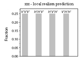
According to local realism the experimental outcome should be as shown in Figure 5. To explain how the local realist prediction is derived, we recall that this position assumes that physical properties exist independent of measurement. Previously it has been shown that eigenvalues of the three‐photon operators according to quantum mechanics are,

\[ \begin{matrix} y_1 y_2 y_3 = y_1 x_2 y_3 = x_1 y_2 y_3 = -1 & x_1 x_2 x_3 = 1 \end{matrix} \nonumber \]

It follows that,

\[ (y_1 y_2 x_3 )(y_1 x_2 y_3)(x_1 y_2 y_3) = -1 \nonumber \]

However, this means that x₁x₂x₃ = -1, because y₁y₁ = y₂y₂ = y₃y₃ = 1. (All of the three-photon operators commute, and therefore can have simultaneous eigenvalues. The commutation relations are shown in the Appendix.) According to the local realist view there are four ways to achieve this result (x₁x₂x₃ = -1) V'V'V', H'H'V', H'V'H' and V'H'H'.

Figure 5.

LR results are contradicted by QM calculation.

\[ \begin{matrix} V'V'V' = \text{submatrix(kronecker(V'N, kronecker(V'N, V'N))},~ 1,~ 8,~ 1,~ 1) (| V'V'V' \Psi |)^2 = 0 \\ H'H'V' = \text{submatrix(kronecker(H'N, kronecker(H'N, V'N))},~ 1,~ 8,~ 1,~ 1) (| H'H'V' \Psi |)^2 = 0 \end{matrix} \nonumber \]

Figure 6 shows that none local realistic predictions are observed at a statistically meaningful level in th GHZ experiment. The quantum mechanical prediction for the xxx experiment agrees with experiment, the local realist prediction doesnʹt.

Figure 6.

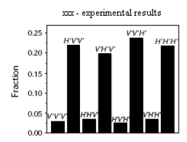
QM calculations confirmed by experimental results.

\[ \begin{matrix} V'V'V' = \text{submatrix(kronecker(V'N, kronecker(V'N, V'N))},~ 1,~ 8,~1,~1) (| V'V'V' \Psi |)^2 = 0 \\ H'V'V' = \text{submatrix(kronecker(H'N, kronecker(V'N, V'N))},~ 1,~ 8,~1,~1) (| H'V'V' \Psi |)^2 = 0.25 \end{matrix} \nonumber \]

For the xxx experiment, the mathematical predictions of quantum mechanics (Figure 4) and the local realist view (Figure 5) when compared with the actual experimental results (Figure 6) present a convincing refutation of local realism.

Appendix

Demonstration that the three‐photon operators commute, allowing for simultaneous eigenvalues.

\[ \begin{matrix} \text{xyy} \text{yxy} - \text{yxy} \text{xyy} \rightarrow 0 & \text{xyy} \text{yyx} - \text{yyx} \text{xyy} \rightarrow 0 & \text{xyy} \text{xxx} - \text{xxx} \text{xyy} \rightarrow 0 \\ \text{yxy} \text{yyx} - \text{yyx} \text{yxy} \rightarrow 0 & \text{yxy} \text{xxx} - \text{xxx} \text{yxy} \rightarrow 0 & \text{yyx} \text{xxx} - \text{xxx} \text{yyx} \rightarrow 0 \end{matrix} \nonumber \]