8.12: Quantum Teleportation - Four Perspectives

The science fiction dream of "beaming" objects from place to place is now a reality - at least for particles of light. Anton Zeilinger, Scientific American, April 2000, page 50.

Quantum teleportation is a way of transferring the state of one particle to a second, effectively teleporting the initial particle. (Tony Sudbery, Nature, December 11, 1997, page 551.)

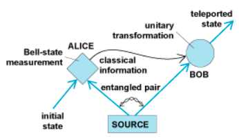
As shown in the graphic below, quantum teleportation is a form of information transfer that requires pre-existing entanglement and a classical communication channel to send information from one location to another.

Alice has the photon to be teleported and a photon of an entangled pair that she shares with Bob. She performs a measurement on her photons that projects them into one of the four Bell states and Bob's photon, via the entangled quantum channel, into a state that has a unique relationship to the state of the teleportee. Bob carries out one of four unitary operations on his photon depending on the results of Alice's measurement, which she sends him through a classical communication channel.

The figure (Nature, December 11, 1997, page 576) on the left provides a graphic summary of the first successful teleportation experiment. The quantum circuit on the right shows a method of implementation.

\[ \begin{matrix} ~ & \text{Initial} ~ & ~ & ~ & ~ \text{Final} \\ ~ & | \Psi \rangle & \cdot & \cdots & \fbox{H} & \triangleright & \text{Measure}~ | \text{a} \rangle ~ \text{0 or 1} \\ \text{Alice} & ~ & | ~ & ~ & ~ & ~ & \text{Bell state measurement} \\ ~ & \cdot & \oplus & \cdots & \cdots & \triangleright & \text{Measure}~ | \text{b} \rangle ~ \text{0 or 1} \\ ~ & \beta_{00} \\ \text{Bob} & \cdot & \cdots & \cdots & \cdots & \triangleright & X^b Z^a \rightarrow | \Psi \rangle \end{matrix} \nonumber \]

The teleportee and the Bell states indexed in binary notation:

Teleportee:

\[ \begin{pmatrix} \sqrt{ \frac{1}{3}} \\ \sqrt{ \frac{2}{3}} \end{pmatrix} \nonumber \]

Bell states:

\[ \begin{matrix} \beta_{00} = \frac{1}{ \sqrt{2}} \begin{pmatrix} 1 \\ 0 \\ 0 \\ 1 \end{pmatrix} & \beta_{01} = \frac{1}{ \sqrt{2}} \begin{pmatrix} 0 \\ 1 \\ 1 \\ 0 \end{pmatrix} & \beta_{10} = \frac{1}{ \sqrt{2}} \begin{pmatrix} 1 \\ 0 \\ 0 \\ -1 \end{pmatrix} & \beta_{11} = \frac{1}{ \sqrt{2}} \begin{pmatrix} 0 \\ 1 \\ -1 \\ 0 \end{pmatrix} \end{matrix} \nonumber \]

Truth tables and matrices representing the various teleportation circuit operations:

\[ \begin{matrix} |0 \rangle = \begin{pmatrix} 1 \\ 0 \end{pmatrix} & |1 \rangle = \begin{pmatrix} 0 \\ 1 \end{pmatrix} & X = \begin{pmatrix} 0~ \text{to} ~1 \\ 1~ \text{to} ~ -1 \end{pmatrix} & H = \begin{bmatrix} 0~ \text{to}~ \frac{(0 + 1)}{ \sqrt{2}} \\ 1~ \text{to}~ \frac{(0 - 1)}{ \sqrt{2}} \end{bmatrix} & \text{CNOT} = \begin{pmatrix} 00~ \text{to} ~00 \\ 01~ \text{to} ~01 \\ 10~ \text{to} ~11 \\ 11~ \text{to} ~10 \end{pmatrix} \end{matrix} \nonumber \]

\[ \begin{matrix} I = \begin{pmatrix} 1 & 0 \\ 0 & 1 \end{pmatrix} & X = \begin{pmatrix} 0 & 1 \\ 1 & 0 \end{pmatrix} & Z = \begin{pmatrix} 1 & 0 \\ 0 & -1 \end{pmatrix} & H = \frac{1}{ \sqrt{2}} \begin{pmatrix} 1 & 1 \\ 1 & -1 \end{pmatrix} & \text{CNOT} = \begin{pmatrix} 1 & 0 & 0 & 0 \\ 0 & 1 & 0 & 0 \\ 0 & 0 & 0 & 1 \\ 0 & 0 & 1 & 0 \end{pmatrix} \end{matrix} \nonumber \]

Perspective I. Using the truth tables, the operation of the teleportation circuit is expressed in Dirac notation.

\[ \left( \sqrt{ \frac{1}{3}} |0 \rangle + \sqrt{ \frac{2}{3}} |1 \rangle \right) \frac{1}{ \sqrt{2}} \left( |00 \rangle + |11 \rangle \right) = \frac{1}{ \sqrt{2}} \left[ \sqrt{ \frac{1}{3}} \left( |00 \rangle |0 \rangle + |01 \rangle |1 \rangle \right) + \sqrt{ \frac{2}{3}} \left( |10 \rangle |0 \rangle + |11 \rangle |1 \rangle \right) \right] \nonumber \]

\( \text{CNOT} \otimes I\)

\[ \frac{1}{ \sqrt{2}} \left[ \sqrt{ \frac{1}{3}} (|00 \rangle |0 \rangle + |01 \rangle |1 \rangle ) + \sqrt{ \frac{2}{3}} (|11 \rangle |0 \rangle + |10 \rangle |1 \rangle ) \right] = \frac{1}{ \sqrt{2}} \left[ \sqrt{ \frac{1}{3}} |0 \rangle (|00 \rangle + |11 \rangle ) + \sqrt{ \frac{2}{3}} |1 \rangle ( |10 \rangle + |01 \rangle ) \right] \nonumber \]

\( H \otimes I \otimes I\)

\[ \frac{1}{2} \left[ \sqrt{ \frac{1}{3}} (|0 \rangle + |1 \rangle ) (|00 \rangle + | 11 \rangle ) + \sqrt{ \frac{2}{3}} (|0 \rangle - |1 \rangle) (|10 \rangle + |01 \rangle ) \right] \nonumber \]

\( \downarrow\)

\[ \frac{1}{2} \left[ |00 \rangle \begin{pmatrix} \sqrt{ \frac{1}{3}} \\ \sqrt{ \frac{2}{3}} \end{pmatrix} + |01 \rangle \begin{pmatrix} \sqrt{ \frac{2}{3}} \\ \sqrt{ \frac{1}{3}} \end{pmatrix} + |10 \rangle \begin{pmatrix} \sqrt{ \frac{1}{3}} \\ - \sqrt{ \frac{2}{3}} \end{pmatrix} + |11 \rangle \begin{pmatrix} - \sqrt{ \frac{2}{3}} \\ \sqrt{ \frac{1}{3}} \end{pmatrix} \right] \xrightarrow{Action} \frac{1}{2} \left[ I \begin{pmatrix} \sqrt{ \frac{1}{3}} \\ \sqrt{ \frac{2}{3}} \end{pmatrix} + X \begin{pmatrix} \sqrt{ \frac{2}{3}} \\ \sqrt{ \frac{1}{3}} \end{pmatrix} + Z \begin{pmatrix} \sqrt{ \frac{1}{3}} \\ - \sqrt{ \frac{2}{3}} \end{pmatrix} + Z X \begin{pmatrix} - \sqrt{ \frac{2}{3}} \\ \sqrt{ \frac{1}{3}} \end{pmatrix} \right] \nonumber \]

Alice's Bell state measurement result (|00>, |01>. |10> or |11>, see indexed Bell states above) determines the operation (I, X, Z or ZX) that Bob performs on his photon.

Perspective II. The three-cubit initial state is re-written as a linear superposition of the four possible Bell states that Alice can find on measurement. Note that this is a equivalent to the expression on the left side of the equation immediately above if the Bell states are replaced by their binary indices, as they would be after the Bell state measurement.

\[ \Psi \rangle = \begin{pmatrix} \sqrt{ \frac{1}{3}} \\ \sqrt{ \frac{2}{3}} \end{pmatrix} \otimes \sqrt{ \frac{1}{2}} \begin{pmatrix} 1 \\ 0 \\ 0 \\ 1 \end{pmatrix} = \sqrt{ \frac{1}{2}} \begin{pmatrix} \sqrt{ \frac{1}{3}} \\ 0 \\ 0 \\ \sqrt{ \frac{1}{3}} \\ \sqrt{ \frac{2}{3}} \\ 0 \\ 0 \\ \sqrt{ \frac{2}{3}} \end{pmatrix} \nonumber \]

\[= \frac{1}{2} \left[ \sqrt{ \frac{1}{2}} \begin{pmatrix} 1 \\ 0 \\ 0 \\ 1 \end{pmatrix} \otimes \begin{pmatrix} \sqrt{ \frac{1}{3}} \\ \sqrt{ \frac{2}{3}} \end{pmatrix} + \sqrt{ \frac{1}{2}} \begin{pmatrix} 0 \\ 1 \\ 1 \\ 0 \end{pmatrix} \otimes \begin{pmatrix} \sqrt{ \frac{2}{3}} \\ \sqrt{ \frac{1}{3}} \end{pmatrix} + \sqrt{ \frac{1}{2}} \begin{pmatrix} 1 \\ 0 \\ 0 \\ -1 \end{pmatrix} \otimes \begin{pmatrix} \sqrt{ \frac{1}{3}} \\ - \sqrt{ \frac{2}{3}} \end{pmatrix} + \sqrt{ \frac{1}{2}} \begin{pmatrix} 0 \\ 1 \\ -1 \\ 0 \end{pmatrix} \otimes \begin{pmatrix} - \sqrt{ \frac{2}{3}} \\ \sqrt{ \frac{1}{3}} \end{pmatrix} \right] \nonumber \]

Condensed version of the equation:

\[ | \Psi \rangle = \begin{pmatrix} \sqrt{ \frac{1}{3}} \\ \sqrt{ \frac{2}{3}} \end{pmatrix} \otimes \beta_{00} = \frac{1}{2} \left[ \beta_{00} \otimes \begin{pmatrix} \sqrt{ \frac{1}{3}} \\ \sqrt{ \frac{2}{3}} \end{pmatrix} + \beta_{01} \otimes \begin{pmatrix} \sqrt{ \frac{2}{3}} \\ \sqrt{ \frac{1}{3}} \end{pmatrix} + \beta_{10} \otimes \begin{pmatrix} \sqrt{ \frac{1}{3}} \\ - \sqrt{ \frac{2}{3}} \end{pmatrix} + \beta_{11} \otimes \begin{pmatrix} - \sqrt{ \frac{2}{3}} \\ \sqrt{ \frac{1}{3}} \end{pmatrix} \right] \nonumber \]

Another way to write the equation:

\[ | \Psi \rangle = \begin{pmatrix} \sqrt{ \frac{1}{3}} \\ \sqrt{ \frac{2}{3}} \end{pmatrix} \otimes \beta_{00} = \frac{1}{2} \left[ \beta_{00} \otimes I \begin{pmatrix} \sqrt{ \frac{1}{3}} \\ \sqrt{ \frac{2}{3}} \end{pmatrix} + \beta_{01} \otimes X \begin{pmatrix} \sqrt{ \frac{1}{3}} \\ \sqrt{ \frac{2}{3}} \end{pmatrix} + \beta_{10} \otimes Z \begin{pmatrix} \sqrt{ \frac{1}{3}} \\ \sqrt{ \frac{2}{3}} \end{pmatrix} + \beta_{11} \otimes XZ \begin{pmatrix} \sqrt{ \frac{1}{3}} \\ \sqrt{ \frac{2}{3}} \end{pmatrix} \right] \nonumber \]

Perspective III. The teleportation circuit (TC) is written as a composite matrix operator which then operates on the initial three-qubit state.

\[ \begin{matrix} \Psi = \frac{1}{ \sqrt{2}} \begin{pmatrix} \sqrt{ \frac{1}{3}} & 0 & 0 & \sqrt{ \frac{1}{3}} \sqrt{ \frac{2}{3}} & 0 & 0 & \sqrt{ \frac{2}{3}} \end{pmatrix}^2 & & \text{TC = kronecker(H, kronecker(I, I)) kronecker(CNOT, I)} \end{matrix} \nonumber \]

After operation of the circuit the system is in a superposition state involving the Bell state indices on the top two registers. The third register contains a state that can easily be transformed into the teleportee once Alice tells Bob which Bell state she observed.

\[ \text{TC} \Psi = \begin{pmatrix} 0.289 \\ 0.408 \\ 0.408 \\ 0.289 \\ 0.289 \\ -0.408 \\ -0.408 \\ 0.289 \end{pmatrix} \begin{array}{l} = \frac{1}{2} \left[ \begin{pmatrix} 1 \\ 0 \end{pmatrix} \otimes \begin{pmatrix} 1 \\ 0 \end{pmatrix} \otimes \begin{pmatrix} \sqrt{ \frac{1}{3}} \\ \sqrt{ \frac{2}{3}} \end{pmatrix} + \begin{pmatrix} 1 \\ 0 \end{pmatrix} \otimes \begin{pmatrix} 0 \\ 1 \end{pmatrix} \otimes \begin{pmatrix} \sqrt{ \frac{2}{3}} \\ \sqrt{ \frac{1}{3}} \end{pmatrix} + \begin{pmatrix} 0 \\ 1 \end{pmatrix} \otimes \begin{pmatrix} 1 \\ 0 \end{pmatrix} \otimes \begin{pmatrix} \sqrt{ \frac{1}{3}} \\ - \sqrt{ \frac{2}{3}} \end{pmatrix} + \begin{pmatrix} 0 \\ 1 \end{pmatrix} \otimes \begin{pmatrix} 0 \\ 1 \end{pmatrix} \otimes \begin{pmatrix} - \sqrt{ \frac{2}{3}} \\ \sqrt{ \frac{1}{3}} \end{pmatrix} \right] \\ = \frac{1}{2} \left[ \begin{pmatrix} 1 \\ 0 \\ 0 \\ 0 \end{pmatrix} \otimes \begin{pmatrix} \sqrt{ \frac{1}{3}} \\ \sqrt{ \frac{2}{3}} \end{pmatrix} + \begin{pmatrix} 0 \\ 1 \\ 0 \\ 0 \end{pmatrix} \otimes \begin{pmatrix} \sqrt{ \frac{2}{3}} \\ \sqrt{ \frac{1}{3}} \end{pmatrix} + \begin{pmatrix} 0 \\ 0 \\ 1 \\ 0 \end{pmatrix} \otimes \begin{pmatrix} \sqrt{ \frac{1}{3}} \\ -\sqrt{ \frac{2}{3}} \end{pmatrix} + \begin{pmatrix} 0 \\ 0 \\ 0 \\ 1 \end{pmatrix} \otimes \begin{pmatrix} - \sqrt{ \frac{2}{3}} \\ \sqrt{ \frac{1}{3}} \end{pmatrix} \right] \end{array} \nonumber \]

Tabular summary of teleportation experiment:

\[ \begin{pmatrix} \text{Alice Measurement Result} & \beta_{00} & \beta_{01} & \beta{10} & \beta_{11} \\ \text{Bob's Action} & I & X & Z & ZX \end{pmatrix} \nonumber \]

Bell state indices:

\[ \begin{matrix} \text{kronecker (H, I) CNOT} \beta_{00} = \begin{pmatrix} 1 \\ 0 \\ 0 \\ 0 \end{pmatrix} & \text{kronecker (H, I) CNOT} \beta_{01} = \begin{pmatrix} 0 \\ 1 \\ 0 \\ 0 \end{pmatrix} \\ \text{kronecker (H, I) CNOT} \beta_{10} = \begin{pmatrix} 0 \\ 0 \\ 1 \\ 0 \end{pmatrix} & \text{kronecker (H, I) CNOT} \beta_{11} = \begin{pmatrix} 0 \\ 0 \\ 0 \\ 1 \end{pmatrix} \end{matrix} \nonumber \]

A similar approach is to use projection operators on the top two qubits to simulate the four measurement outcomes. See the Appendix for more on this method.

\[ \begin{matrix} ~& ~ & \text{Bob's Action} \\ \text{Measure} |00 \rangle & 2 \text{kronecker} \left[ \begin{pmatrix} 1 \\ 0 \end{pmatrix} \begin{pmatrix} 1 \\ 0 \end{pmatrix} ^T, \text{kronecker} \left[ \begin{pmatrix} 1 \\ 0 \end{pmatrix} \begin{pmatrix} 1 \\ 0 \end{pmatrix} ^T, I \right] \right] \text{TC} \Psi = \begin{pmatrix} 0.577 \\ 0.816 \\ 0 \\ 0 \\ 0 \\ 0 \\ 0 \\ 0 \end{pmatrix} & \text{No action required} \\ \text{Measure} |01 \rangle & 2 \text{kronecker} \left[ \begin{pmatrix} 1 \\ 0 \end{pmatrix} \begin{pmatrix} 1 \\ 0 \end{pmatrix} ^T, \text{kronecker} \left[ \begin{pmatrix} 0 \\ 1 \end{pmatrix} \begin{pmatrix} 0 \\ 1 \end{pmatrix} ^T, I \right] \right] \text{TC} \Psi = \begin{pmatrix} 0 \\ 0 \\ 0.816 \\ 0.577 \\ 0 \\ 0 \\ 0 \\ 0 \end{pmatrix} & \text{Operate with X} \\ \text{Measure} |10 \rangle & 2 \text{kronecker} \left[ \begin{pmatrix} 0 \\ 1 \end{pmatrix} \begin{pmatrix} 0 \\ 1 \end{pmatrix} ^T, \text{kronecker} \left[ \begin{pmatrix} 1 \\ 0 \end{pmatrix} \begin{pmatrix} 1 \\ 0 \end{pmatrix} ^T, I \right] \right] \text{TC} \Psi = \begin{pmatrix} 0 \\ 0 \\ 0 \\ 0 \\ 0.577 \\ -0.816 \\ 0 \\ 0 \end{pmatrix} & \text{Operate with Z} \\ \text{Measure} |11 \rangle & 2 \text{kronecker} \left[ \begin{pmatrix} 0 \\ 1 \end{pmatrix} \begin{pmatrix} 0 \\ 1 \end{pmatrix} ^T, \text{kronecker} \left[ \begin{pmatrix} 0 \\ 1 \end{pmatrix} \begin{pmatrix} 0 \\ 1 \end{pmatrix} ^T, I \right] \right] \text{TC} \Psi = \begin{pmatrix} 0 \\ 0 \\ 0 \\ 0 \\ 0 \\ 0 \\ -0.816 \\ 0.577 \end{pmatrix} & \text{Operate with ZX} \end{matrix} \nonumber \]

Perspective IV. Projecting the teleportee photon 1 (green) onto the result of Alice's Bell state measurement (blue) yields the state of photon 2 which was initially entangled with Bob's photon 3. Projection of this state onto the original 2-3 entangled state (red) transforms Bob's photon to the teleportee state 25% of the time. As is now shown this happens when Alice's Bell state measurment yields β₀₀.

\[ _{12} \langle \beta_{00} | \Psi \rangle_1 | \beta_{00} \rangle_{23} = \frac{1}{ \sqrt{2}} \left[ \begin{pmatrix} 1 \\ 0 \end{pmatrix}_1 ^T \otimes \begin{pmatrix} 1 \\ 0 \end{pmatrix} _2 ^T + \begin{pmatrix} 0 \\ 1 \end{pmatrix} _1 ^T \otimes \begin{pmatrix} 0 \\ 1 \end{pmatrix} _2 ^T\right] \begin{pmatrix} \sqrt{ \frac{1}{3}} \\ \sqrt{ \frac{2}{3}} \end{pmatrix}_1 \frac{1}{ \sqrt{2}} \left[ \begin{pmatrix} 1 \\ 0 \end{pmatrix}_2 \otimes \begin{pmatrix} 1 \\ 0 \end{pmatrix}_3 + \begin{pmatrix} 0 \\ 1 \end{pmatrix}_2 \otimes \begin{pmatrix} 0 \\ 1 \end{pmatrix}_3 \right]= \frac{1}{2} \begin{pmatrix} \sqrt{ \frac{1}{3}} \\ \sqrt{ \frac{2}{3}} \end{pmatrix}_3 \nonumber \]

An algebraic analysis of this example is as follows.

\( \text{Teleportee}\)

\[ \frac{1}{ \sqrt{2}} \left[ _1 \langle 0|_2 \langle 0| +~ _1 \langle 1|_2 \langle 1| \right] \left[ \alpha |0 \rangle_1 + \beta |1 \rangle_1 \right] \frac{1}{ \sqrt{2}} \left[ |0 \rangle_2 |0 \rangle_3 + |1 \rangle_2 |1 \rangle_3 \right] \nonumber \]

\( \downarrow\)

\[ \frac{1}{ \sqrt{2}} \left[ \alpha _2 \langle 0| + \beta _2 \langle 1| \right] \frac{1}{ \sqrt{2}} \left[ |0 \rangle_2 |0 \rangle_3 + |1 \rangle_2 |1 \rangle_3 \right] \nonumber \]

\( \downarrow\)

\[ \frac{1}{2} \left[ \alpha |0 \rangle_3 + \beta |1 \rangle_3 \right] \nonumber \]

Naturally this approach yields the same results as the previous perspectives when Alice's Bell state measurement is β₀₁, β₁₀ and β₁₁. As demonstrated previously for these results Bob's action is X, Z and ZX, respectively.

\[ _{12} \langle \beta_{01} | \Psi \rangle_1 | \beta_{00} \rangle_{23} = \frac{1}{ \sqrt{2}} \left[ \begin{pmatrix} 1 \\ 0 \end{pmatrix}_1 ^T \otimes \begin{pmatrix} 0 \\ 1 \end{pmatrix} _2 ^T + \begin{pmatrix} 0 \\ 1 \end{pmatrix} _1 ^T \otimes \begin{pmatrix} 1 \\ 0 \end{pmatrix} _2 ^T\right] \begin{pmatrix} \sqrt{ \frac{1}{3}} \\ \sqrt{ \frac{2}{3}} \end{pmatrix}_1 \frac{1}{ \sqrt{2}} \left[ \begin{pmatrix} 1 \\ 0 \end{pmatrix}_2 \otimes \begin{pmatrix} 1 \\ 0 \end{pmatrix}_3 + \begin{pmatrix} 0 \\ 1 \end{pmatrix}_2 \otimes \begin{pmatrix} 0 \\ 1 \end{pmatrix}_3 \right]= \frac{1}{2} \begin{pmatrix} \sqrt{ \frac{2}{3}} \\ \sqrt{ \frac{1}{3}} \end{pmatrix}_3 \nonumber \]

\[ _{12} \langle \beta_{10} | \Psi \rangle_1 | \beta_{00} \rangle_{23} = \frac{1}{ \sqrt{2}} \left[ \begin{pmatrix} 1 \\ 0 \end{pmatrix}_1 ^T \otimes \begin{pmatrix} 1 \\ 0 \end{pmatrix} _2 ^T - \begin{pmatrix} 0 \\ 1 \end{pmatrix} _1 ^T \otimes \begin{pmatrix} 0 \\ 1 \end{pmatrix} _2 ^T\right] \begin{pmatrix} \sqrt{ \frac{1}{3}} \\ \sqrt{ \frac{2}{3}} \end{pmatrix}_1 \frac{1}{ \sqrt{2}} \left[ \begin{pmatrix} 1 \\ 0 \end{pmatrix}_2 \otimes \begin{pmatrix} 1 \\ 0 \end{pmatrix}_3 + \begin{pmatrix} 0 \\ 1 \end{pmatrix}_2 \otimes \begin{pmatrix} 0 \\ 1 \end{pmatrix}_3 \right]= \frac{1}{2} \begin{pmatrix} \sqrt{ \frac{1}{3}} \\ - \sqrt{ \frac{2}{3}} \end{pmatrix}_3 \nonumber \]

\[ _{12} \langle \beta_{11} | \Psi \rangle_1 | \beta_{00} \rangle_{23} = \frac{1}{ \sqrt{2}} \left[ \begin{pmatrix} 1 \\ 0 \end{pmatrix}_1 ^T \otimes \begin{pmatrix} 0 \\ 1 \end{pmatrix} _2 ^T - \begin{pmatrix} 0 \\ 1 \end{pmatrix} _1 ^T \otimes \begin{pmatrix} 1 \\ 0 \end{pmatrix} _2 ^T\right] \begin{pmatrix} \sqrt{ \frac{1}{3}} \\ \sqrt{ \frac{2}{3}} \end{pmatrix}_1 \frac{1}{ \sqrt{2}} \left[ \begin{pmatrix} 1 \\ 0 \end{pmatrix}_2 \otimes \begin{pmatrix} 1 \\ 0 \end{pmatrix}_3 + \begin{pmatrix} 0 \\ 1 \end{pmatrix}_2 \otimes \begin{pmatrix} 0 \\ 1 \end{pmatrix}_3 \right]= \frac{1}{2} \begin{pmatrix} - \sqrt{ \frac{2}{3}} \\ \sqrt{ \frac{1}{3}} \end{pmatrix}_3 \nonumber \]

Summary of the quantum teleportation protocol: "Quantum teleportation provides a 'disembodied' way to tranfer quantum states from one object to another at a distant location, assisted by previously shared entangled states and a classical communication channel." Nature 518, 516 (2015)

The paper cited above reported the first successful teleportation of two degrees of freedom of a single photon. The analysis is somewhat more complicated than that provided in this tutorial, but the general principle is the same. The quantum channel is a hyper-entangled state shared by Alice and Bob, rather than one of the simple entangled Bell states.

Appendix

Addendum to Perspective III. In these calculations the required operations by Bob are actually carried out on the third qubit.

\[ \begin{matrix} \text{Measure} |00 \rangle ~ \text{do nothing} & \text{kronecker(I, kronecker(I, I)) 2 kronecker} \left[ \begin{pmatrix} 1 \\ 0 \end{pmatrix} \begin{pmatrix} 1 \\ 0 \end{pmatrix} ^T, \text{kronecker} \left[ \begin{pmatrix} 1 \\ 0 \end{pmatrix} \begin{pmatrix} 1 \\ 0 \end{pmatrix} ^T, I \right] \right] \text{TC} \Psi = \begin{pmatrix} 0.577 \\ 0.816 \\ 0 \\ 0 \\ 0 \\ 0 \\ 0 \\ 0 \end{pmatrix} \\ \text{Measure} |01 \rangle ~ \text{operate with X} & \text{kronecker(I, kronecker(I, X)) 2 kronecker} \left[ \begin{pmatrix} 1 \\ 0 \end{pmatrix} \begin{pmatrix} 1 \\ 0 \end{pmatrix} ^T, \text{kronecker} \left[ \begin{pmatrix} 0 \\ 1 \end{pmatrix} \begin{pmatrix} 0 \\ 1 \end{pmatrix} ^T, I \right] \right] \text{TC} \Psi = \begin{pmatrix} 0 \\ 0 \\ 0.577 \\ 0.816 \\ 0 \\ 0 \\ 0 \\ 0 \end{pmatrix} \\ \text{Measure} |10 \rangle ~ \text{operate with Z} & \text{kronecker(I, kronecker(I, Z)) 2 kronecker} \left[ \begin{pmatrix} 0 \\ 1 \end{pmatrix} \begin{pmatrix} 0 \\ 1 \end{pmatrix} ^T, \text{kronecker} \left[ \begin{pmatrix} 1 \\ 0 \end{pmatrix} \begin{pmatrix} 1 \\ 0 \end{pmatrix} ^T, I \right] \right] \text{TC} \Psi = \begin{pmatrix} 0 \\ 0 \\ 0 \\ 0 \\ 0.577 \\ 0.816 \\ 0 \\ 0 \end{pmatrix} \\ \text{Measure} |11 \rangle ~ \text{operate with Z} & \text{kronecker(I, kronecker(I, Z, X)) 2 kronecker} \left[ \begin{pmatrix} 0 \\ 1 \end{pmatrix} \begin{pmatrix} 0 \\ 1 \end{pmatrix} ^T, \text{kronecker} \left[ \begin{pmatrix} 0 \\ 1 \end{pmatrix} \begin{pmatrix} 0 \\ 1 \end{pmatrix} ^T, I \right] \right] \text{TC} \Psi = \begin{pmatrix} 0 \\ 0 \\ 0 \\ 0 \\ 0 \\ 0 \\ 0.577 \\ 0.816 \end{pmatrix} \end{matrix} \nonumber \]