8.2: Quantum Teleportation - A Brief Introduction

Alice wishes to teleport a photon in the polarization state, αh₁ + βv₁, to Bob, where α and β are complex coefficients such that the sum of the square of their absolute magnitudes is unity. The letters h and v refer to the vertical and horizontal polarization states. In preparation for the teleportation event, Alice and Bob first prepare an entangled state involving photons 2 and 3, \( \frac{ h_2 v_3 - v_2 h_3}{ \sqrt{2}}\), as shown in the figure below [Nature 390, 576 (1997)].

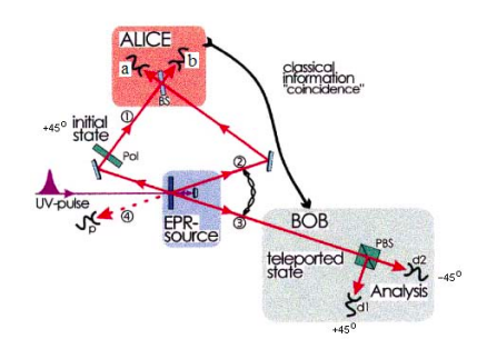
Alice has photon 2 and Bob photon 3, but because they are in an entangled state the photons do not have well‐defined individual polarization states.

Alice arranges for photons 1 and 2 to arrive at opposite sides of a beam splitter at the same time. This gives rise to the following state,

\[ ( \alpha h_1 \beta v_1 ) \frac{h_2 v_3 - v_2 h_3}{ \sqrt{2}} \nonumber \]

which upon expansion yields,

\[ \frac{1}{2} \sqrt{2} \alpha h_1 h_2 v_3 - \frac{1}{2} \alpha h_1 v_2 h_3 + \frac{1}{2} \beta v_1 h_2 v_3 - \frac{1}{2} \beta v_1 v_2 h_3 \nonumber \]

Alice now makes a Bell‐state measurement (vide infra) at the detectors (a and b) to the left and right of her beam splitter. Bell states are the four maximally entangled h‐v polarization states of photons 1 and 2. They are as follows:

\[ \Phi_p = \frac{h_1 h_2 + v_1 v_2}{ \sqrt{2}} ~~~ \Phi_m = \frac{h_1 h_2 - v_1 v_2}{ \sqrt{2}} ~~~ \Psi_p = \frac{h_1 v_2 + v_1 h_2}{ \sqrt{2}} ~~~ \Psi_m = \frac{h_1 v_2 - v_1 h_2}{ \sqrt{2}} \nonumber \]

The products of the polarization states of photons 1 and 2 in equation (3) can be expressed as linear superpositions of the Bell states.

\[ h_1 h_2 = \frac{ \sqrt{2}}{2} ( \Phi_p + \Phi_m) ~~~ h_1 v_2 = \frac{ \sqrt{2}}{2} ( \Psi_p + \Psi_m) ~~~ v_1 h_2 = \frac{ \sqrt{2}}{2} ( \Psi_p - \Psi_m) ~~~ v_1 v_2 = \frac{ \sqrt{2}}{2} ( \Phi_p - \Phi_m) \nonumber \]

We can let Mathcad do the heavy lifting by having it expand (1), substitute equations (4) and collect on the Bell states.

\[ ( \alpha h_1 \beta v_1) \frac{h_2v_3 - v_2 h_3}{ \sqrt{2}} \begin{array}{|l}
\text{expand} \\
\text{substitute}, h_1 h_2 = \frac{ \sqrt{2}}{2} ( \Phi_p + \Phi_m) \\
\text{substitute}, h_1 v_2 = \frac{ \sqrt{2}}{2} ( \Psi_p + \Psi_m) \rightarrow \left( \frac{ \beta h_3}{2} + \frac{ \alpha v_3}{2} \right) \Phi_m + \left( \frac{ \alpha v_3}{2} - \frac{ \beta h_3}{2} \right) \Phi_p + \left( - \frac{ \alpha h_3}{2} - \frac{ \beta v_3}{2} \right) \Psi_m + \left( \frac{ \beta v_3}{2} - \frac{ \alpha h_3}{2} \right) \Psi_p \\
\text{substitute}, v_1 h_2 = \frac{ \sqrt{2}}{2} ( \Psi_p - \Psi_m) \\
\text{substitute}, v_1 v_2 = \frac{ \sqrt{2}}{2} ( \Phi_p - \Phi_m) \\
\text{collect},~ \Phi_m,~ \Phi_p,~ \Psi_m,~ \Psi_p \\
\end{array} \nonumber \]

Thus Aliceʹs Bell‐state measurement has four equally likely (0.5² = 0.25) outcomes. We will restrict our attention to the third term which says that if Alice measures Ψ_m, then Bob receives photon 1ʹs polarization state without further action by him.

\[ - ( \alpha h_3 + \beta v_3 ) \Psi_m \nonumber \]

This will occur 25% of the time. The other three possible measurement outcomes are more complicated to analyze and will not be discussed further here. So we assume Alice measures Ψ_m and communicates this to Bob by classical means so that he knows that his photon (#3) now has the polarization state of the original photon 1. But, how does Alice know that the results she observes at detectors a and b mean that photons 1 and 2 are in Bell state Ψ_m?

First the short, qualitative answer. Of the four Bell states, Ψ_m is the only one that is antisymmetric with respect to the interchange of the labels of the photons. Thus, in spite of the fact that photons individually are bosons, this entangled state is fermionic ‐ collectively the photons are behaving as fermions. This means that they canʹt be in the same (measurement) state at the same time. If photon 1 is detected at a, then photon 2 will be detected at b. Therefore, if Alice observes a‐b coincidences it means that photons 1 and 2 are in the Ψ_m Bell state and photon 1ʹs polarization state has been teleported to Bobʹs photon (#3).

Bob confirms that he has received the polarization state of photon 1 using a polarizing beam splitter as shown in the figure above. Suppose Alice encodes photon 1 with a 45o polarization, then Bob sets his polarizing beam splitter to detect +45^o/‐45^o polarized photons. A three‐fold coincidence between detectors a, b and Bobʹs +45^o detector confirms teleportation. This was procedure employed in the original experiment published in Nature on December 11, 1997.

It should be pointed out that the initial entangled state used by Alice and Bob involving photons 2 and 3 is the Bell state Ψ_m. As was just seen, if Alice observes Ψ_m in her Bell‐state measurement Bob receives photon 1ʹs polarization state without further action by him. As is shown below the analogous thing occurs if the initial entangled state is Ψ_p, Φ_p or Φ_m.

\[ \Psi_p > \left( \frac{ \alpha h_3}{2} + \frac{ \beta v_3}{2} \right) \Psi_p \nonumber \]

\[ ( \alpha h_1 \beta v_1) \frac{h_2v_3 + v_2 h_3}{ \sqrt{2}} \begin{array}{|l}
\text{expand} \\
\text{substitute}, h_1 h_2 = \frac{ \sqrt{2}}{2} ( \Phi_p + \Phi_m) \\
\text{substitute}, h_1 v_2 = \frac{ \sqrt{2}}{2} ( \Psi_p + \Psi_m) \rightarrow \left( \frac{ \alpha v_3}{2} - \frac{ \beta h_3}{2} \right) \Phi_m + \left( \frac{ \beta h_3}{2} + \frac{ \alpha v_3}{2} \right) \Phi_p + \left( \frac{ \alpha h_3}{2} - \frac{ \beta v_3}{2} \right) \Psi_m + \left( \frac{ \alpha h_3}{2} + \frac{ \beta v_3}{2} \right) \Psi_p \\
\text{substitute}, v_1 h_2 = \frac{ \sqrt{2}}{2} ( \Psi_p - \Psi_m) \\
\text{substitute}, v_1 v_2 = \frac{ \sqrt{2}}{2} ( \Phi_p - \Phi_m) \\
\text{collect},~ \Phi_m,~ \Phi_p,~ \Psi_m,~ \Psi_p \\
\end{array} \nonumber \]

\[ \Phi_p > \left( \frac{ \alpha h_3}{2} + \frac{ \beta v_3}{2} \right) \Phi_p \nonumber \]

\[ ( \alpha h_1 \beta v_1) \frac{h_2 h_3 + v_2 v_3}{ \sqrt{2}} \begin{array}{|l}
\text{expand} \\
\text{substitute}, h_1 h_2 = \frac{ \sqrt{2}}{2} ( \Phi_p + \Phi_m) \\
\text{substitute}, h_1 v_2 = \frac{ \sqrt{2}}{2} ( \Psi_p + \Psi_m) \rightarrow \left( \frac{ \alpha h_3}{2} - \frac{ \beta v_3}{2} \right) \Phi_m + \left( \frac{ \alpha h_3}{2} + \frac{ \beta v_3}{2} \right) \Phi_p + \left( \frac{ \alpha v_3}{2} - \frac{ \beta h_3}{2} \right) \Psi_m + \left( \frac{ \beta h_3}{2} + \frac{ \alpha v_3}{2} \right) \Psi_p \\
\text{substitute}, v_1 h_2 = \frac{ \sqrt{2}}{2} ( \Psi_p - \Psi_m) \\
\text{substitute}, v_1 v_2 = \frac{ \sqrt{2}}{2} ( \Phi_p - \Phi_m) \\
\text{collect},~ \Phi_m,~ \Phi_p,~ \Psi_m,~ \Psi_p \\
\end{array} \nonumber \]

\[ \Phi_m > \left( \frac{ \alpha h_3}{2} + \frac{ \beta v_3}{2} \right) \Phi_m \nonumber \]

\[ ( \alpha h_1 \beta v_1) \frac{h_2 h_3 + v_2 v_3}{ \sqrt{2}} \begin{array}{|l}
\text{expand} \\
\text{substitute}, h_1 h_2 = \frac{ \sqrt{2}}{2} ( \Phi_p + \Phi_m) \\
\text{substitute}, h_1 v_2 = \frac{ \sqrt{2}}{2} ( \Psi_p + \Psi_m) \rightarrow \left( \frac{ \alpha h_3}{2} + \frac{ \beta v_3}{2} \right) \Phi_m + \left( \frac{ \alpha h_3}{2} - \frac{ \beta v_3}{2} \right) \Phi_p + \left( - \frac{ \beta h_3}{2} - \frac{ \alpha v_3}{2} \right) \Psi_m + \left( \frac{ \beta h_3}{2} - \frac{ \alpha v_3}{2} \right) \Psi_p \\
\text{substitute}, v_1 h_2 = \frac{ \sqrt{2}}{2} ( \Psi_p - \Psi_m) \\
\text{substitute}, v_1 v_2 = \frac{ \sqrt{2}}{2} ( \Phi_p - \Phi_m) \\
\text{collect},~ \Phi_m,~ \Phi_p,~ \Psi_m,~ \Psi_p \\
\end{array} \nonumber \]