7.41: A Quantum Delayed-Choice Experiment

This tutorial works through the first half of the Science report (Nov. 2, 2012, pp . 634‐637) by Peruzzo et al. with the title given above. The Wheeler‐type delayed‐choice experiment dealt with in this paper is shown schematically in the figure below. An observer has the option of inserting or removing a second beam splitter (BS) in a Mach‐Zehnder interferometer (MZI) after a photon has passed the first BS.

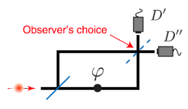
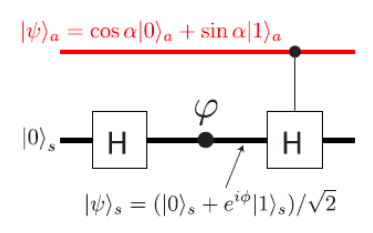
This apparatus is implemented using Hadamard and controlled‐Hadamard gates as shown below. A phase shift is also possible in the lower arm of the interferometer. The operation of the second Hadamard gate is controlled by an ancillary photon which can be prepared as a superposition. For this reason the second beam splitter is called a quantum beam splitter (QBS).

The Hadamard gate is a single‐photon gate as is the phase shifter, while the controlled‐Hadamard gate is a two‐photon gate. Their matrix representations are as follows.

\[ H = \frac{1}{ \sqrt{2}} \begin{pmatrix} 1 & 1 \\ 1 & -1 \end{pmatrix} \nonumber \]

\[ A ( \phi ) = \begin{pmatrix} 1 & 0 \\ 0 & e^{ i \phi} \end{pmatrix} \nonumber \]

\[ A ( \phi ) H \begin{pmatrix} 1 \\ 0 \end{pmatrix} \rightarrow \begin{pmatrix} \frac{ \sqrt{2}}{2} \\ \frac{ \sqrt{2} e^{ \phi i}}{2} \end{pmatrix} \nonumber \]

\[ CH = \begin{pmatrix} 1 & 0 & & 0 & 0 \\ 0 & 1 & 0 & 0 \\ 0 & 0 & \frac{1}{ \sqrt{2}} & \frac{1}{ \sqrt{2}} \\ 0 & 0 & \frac{1}{ \sqrt{2}} & \frac{-1}{ \sqrt{2}} \end{pmatrix} \nonumber \]

The H gate and the phase‐shifter create the superposition at the point of the arrow (see highlighted area above), just before the CH gate. This is the point at which this analysis begins. Using vector tensor multiplication, the composite state (a = ancilla; s = system) is shown below.

\[ \begin{pmatrix} \cos \alpha \\ \sin \alpha \end{pmatrix}_a \otimes \frac{1}{ \sqrt{2}} \begin{pmatrix} 1 \\ e^{i \phi} \end{pmatrix} = \frac{1}{ \sqrt{2}} \begin{pmatrix} \cos \alpha \\ \cos \alpha e^{i \phi} \\ \sin \alpha \\ \sin \alpha e^{i \phi} \end{pmatrix} \nonumber \]

The four output states expressed in the |0 > ‐ |1 > basis are as follows.

\[ | 0 \rangle_a |0 \rangle_s = \begin{pmatrix} 1 \\ 0 \end{pmatrix}_a \otimes \begin{pmatrix} 1 \\ 0 \end{pmatrix}_s = \begin{pmatrix} 1 \\ 0 \\ 0 \\ 0 \end{pmatrix} \nonumber \]

\[ | 1 \rangle_a |0 \rangle_s = \begin{pmatrix} 0 \\ 1 \end{pmatrix}_a \otimes \begin{pmatrix} 1 \\ 0 \end{pmatrix}_s = \begin{pmatrix} 0 \\ 0 \\ 1 \\ 0 \end{pmatrix} \nonumber \]

\[ | 0 \rangle_a |1 \rangle_s = \begin{pmatrix} 1 \\ 0 \end{pmatrix}_a \otimes \begin{pmatrix} 0 \\ 1 \end{pmatrix}_s = \begin{pmatrix} 0 \\ 1 \\ 0 \\ 0 \end{pmatrix} \nonumber \]

\[ | 1 \rangle_a |1 \rangle_s = \begin{pmatrix} 0 \\ 1 \end{pmatrix}_a \otimes \begin{pmatrix} 0 \\ 1 \end{pmatrix}_s = \begin{pmatrix} 0 \\ 0 \\ 0 \\ 1 \end{pmatrix} \nonumber \]

The probability that the photon is detected at Dʹʹ (|0 >s) is:

\[ D" ( \alpha , \phi ) = \left[ \left| \begin{pmatrix} 1 \\ 0 \\ 0 \\ 0 \end{pmatrix} ^T CH \frac{1}{ \sqrt{2}} \begin{pmatrix} \cos \alpha \\ \cos \alpha e^{i \phi} \\ \sin \alpha \\ \sin \alpha e^{i \phi} \end{pmatrix} \right| \right]^2 + \left[ \left| \begin{pmatrix} 0 \\ 0 \\ 1 \\ 0 \end{pmatrix} ^T CH \frac{1}{ \sqrt{2}} \begin{pmatrix} \cos \alpha \\ \cos \alpha e^{i \phi} \\ \sin \alpha \\ \sin \alpha e^{i \phi} \end{pmatrix} \right| \right]^2 \nonumber \]

The probability that the photon is detected at Dʹ (|1 >s) is:

\[ D' ( \alpha , \phi ) = \left[ \left| \begin{pmatrix} 0 \\ 1 \\ 0 \\ 0 \end{pmatrix} ^T CH \frac{1}{ \sqrt{2}} \begin{pmatrix} \cos \alpha \\ \cos \alpha e^{i \phi} \\ \sin \alpha \\ \sin \alpha e^{i \phi} \end{pmatrix} \right| \right]^2 + \left[ \left| \begin{pmatrix} 0 \\ 0 \\ 0 \\ 1 \end{pmatrix} ^T CH \frac{1}{ \sqrt{2}} \begin{pmatrix} \cos \alpha \\ \cos \alpha e^{i \phi} \\ \sin \alpha \\ \sin \alpha e^{i \phi} \end{pmatrix} \right| \right]^2 \nonumber \]

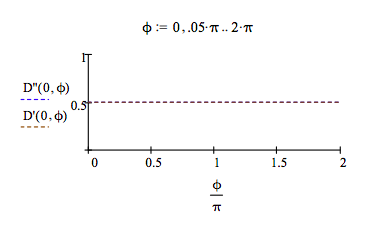
The following graph shows that if α = 0 (the ancillary photon is in the |0 > state), the interferometer is open and the detectors each fire 50% of the time no matter what phase relationship exists between the arms of the interferometer.

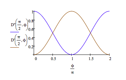
However, if α = π/2 (the ancillary photon is in the |1 > state) the interferometer is closed and interference is observed. The firing of the detectors depends upon the phase relation between the two arms of the interferometer. If ϕ = 0 only Dʹʹ fires, while if ϕ = π only Dʹ fires. As shown below, at other ϕ values both detectors fire.

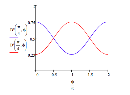
If α = π/4 (the ancilla photon is in a 50‐50 superposition of |0 > and |1 >), both detectors fire at all ϕ values.

Figure 3B are reproduced.

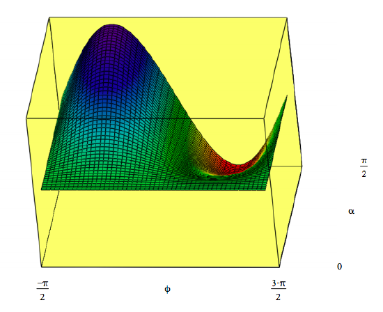
\( N = 50 ~~~ i = 0 .. N ~~~ j = 0 .. N ~~~ \alpha_1 = \frac{ \frac{ \pi}{2} i}{N} ~~~ \phi_j = \frac{ - \pi}{2} + \frac{2 \pi j}{N} ~~~ I_{i,~j} = D'( \alpha_i , \phi_j) \)

In summary, according to Peruzzo et al. this is a delayed‐choice experiment for 0 < α < π/2 because the system photon is in the interferometer before it becomes entangled with the ancillary photon.

While this work represents an exquisite experimental tour de force, in my opinion it doesnʹt reveal anything more about wave‐particle duality than any other quantum optics experiment. We always measure particles (detectors click, photographic film is darkened, etc.), but we interpret what happened or predict what will happen by assuming wavelike behavior. In other words, quantum particles exhibit both wave and particle properties in every experiment. To paraphrase Nick Herbert (Quantum Reality), particles are always detected, but the experimental results observed are the result of wavelike behavior. Richard Feynman put it this way (The Character of Physical Law), ʺI will summarize, then, by saying that electrons arrive in lumps, like particles, but the probability of arrival of these lumps is determined as the intensity of waves would be. It is in this sense that the electron behaves sometimes like a particle and sometimes like a wave. It behaves in two different ways at the same time.ʺ Bragg said, ʺEverything in the future is a wave, everything in the past is a particle.ʺ

In 1951 in his treatise Quantum Theory, David Bohm described wave‐particle duality as follows: ʺOne of the most characteristic features of the quantum theory is the wave‐particle duality, i.e. the ability of matter or light quanta to demonstrate the wave‐like property of interference, and yet to appear subsequently in the form of localiziable particles, even after such interference has taken place.ʺ In other words, to explain interference phenomena wave properties must be assigned to matter and light quanta prior to detection as particles.

Equation (1) in this paper is not a ʺparticleʺ wave function, it is a superposition of the photon being in both arms of the interferometer. It is a wave function (period) and it accurately predicts the future detection results in both the absence and presence of the second beam splitter. See the Appendix for further comment. John Wheeler, designer of several delayed‐choice experiments (both terrestrial and cosmological), had the following to say about the interpretation of such experiments.

... in a loose way of speaking, we decide what the photon shall have done after it has already done it. In actuality it is wrong to talk of the ʹrouteʹ of the photon. For a proper way of speaking we recall once more that it makes no sense to talk of a phenomenon until it has been brought to a close by an irreversible act of amplification. ʹNo elementary phenomenon is a phenomenon until it is a registered (observed) phenomenon.ʹ

This statement was given a convincing and amusing graphical representation by Field Gilbertʹs sketch of Wheelerʹs ʹGreat Smokey Dragonʹ which can be found on page 154 of Jim Baggotʹs The Meaning of Quantum Theory.

Heisenberg said pretty much the same thing as Wheeler when he wrote in 1958: ʺIf we want to describe what happens in an atomic event, we have to realize that the word ʹhappensʹ can only apply to the observation, not to the state of affairs between two observations.ʺ

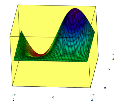
I would also like to point out that equation (4) is mislabeled. The authors claim it is the detection probability at Dʹ as a function of α and ϕ. However, the plot below shows that designation is not consistent with Figure 3B. Equation (4) is actually the detection probability at detector Dʹʹ.

\[ \ln ( \alpha , \phi ) = \frac{1}{2} \cos \alpha ^2 + \cos \left( \frac{ \phi }{2} \right)^2 \sin \alpha ^2 ~~~ I_{i,~j} = \ln ( \alpha_i , \phi_j ) \nonumber \]

Appendix

Removing the phase shifter makes it easier to follow the evolution of the photons through the interferometer and to evaluate the authorsʹ claim that they have demonstrated wave‐particle duality as indicated in their equations 1, 2 and 3. We begin with the composite state prior to the controlled Hadamard gate.

\[ \begin{pmatrix} \cos \alpha \\ \sin \alpha \end{pmatrix} _a \otimes \frac{1}{ \sqrt{2}} \begin{pmatrix} 1 \\ 1 \end{pmatrix} _s = \frac{ \cos \alpha |0 \rangle_a (0| \rangle_s + |1 \rangle_s ) + \sin \alpha |1 \rangle_a (|0 \rangle_s + |1 \rangle_s )}{ \sqrt{2}} \nonumber \]

The operation of the controlled Hadamard (CH) gate is written algebraically.

\[ CH | 0 \rangle_a | 0 \rangle_s = |0 \rangle_a |0 \rangle_s \nonumber \]

\[ CH|0 \rangle_a |1 \rangle_s = |0 \rangle_a |1 \rangle_s \nonumber \]

\[ CH |1 \rangle_a |0 \rangle_s = |1 \rangle_a \frac{1}{ \sqrt{2}} (|0 \rangle_s + |1 \rangle_s) \nonumber \]

\[ CH | 1 \rangle_a |1 \rangle_s = |1 \rangle_a \frac{1}{ \sqrt{2}} (|0 \rangle_s - |1 \rangle_s) \nonumber \]

The action of the controlled Hadamard gate leads to the following state which shows a superposition in blue and interference in red, depending on the state of the control qubit.

\[ \frac{ \cos \alpha |) \rangle_a (|0 \rangle_s + |1 \rangle_s) + \sin \alpha |1 \rangle_a \left( \frac{|0 \rangle_s + |1 \rangle_s}{ \sqrt{2}} + \frac{|0 \rangle_s - |1 \rangle_s}{ \sqrt{2}} \right)}{ \sqrt{2}} = \cos \alpha |0 \rangle_a \frac{|0 \rangle_s + |1 \rangle_s}{ \sqrt{2}} + \sin \alpha |1 \rangle_a |0 \rangle_s \nonumber \]

According to Peruzzo et al. this leads to the following interpretive equation expressing their view of wave‐particle duality.

\[ \cos \alpha | 0 \rangle_a \Psi ( \text{particle}) \rangle_s + \sin \alpha |1 \rangle_a| \Psi ( \text{wave}) \rangle_s \nonumber \]

My objection is that a superposition, even if it dosenʹt lead to interference, is an example of wavelike (delocalized) behavior. The fact that the superposition doesnʹt lead to interference doesnʹt mean the photon took a particular path to a particular detector, it simply means on observation the superposition collapsed with appropriate probability at that detector.

Quantum mechanical entities (quons) do not, as Peruzzo et al. assert, exhibit particle‐ or wavelike behavior depending on the design of the experimental apparatus they encounter. As Bohm, Feynman and Herbert have said quons exhibit wave and particle characteristics in every experiment.