7.40: Another Example of a Two-photon Quantum Eraser

Greenberger, Horne and Zeilinger (GHZ) surveyed the then relatively new field of multiparticle interferometry in an August 1993 Physics Today article, ʺMultiparticle Interferometry and the Superposition Principle.ʺ This tutorial will use Mathcad and tensor algebra to analyze the results associated with Figure 5, which dealt with a two‐photon quantum eraser. A parametric down converter (PDC) produces two horizontally polarized, entangled photons, one taking the upper path and the other the lower path. The beams are combined at a beam splitter as shown below.

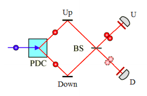
As the figure shows both photons arrive at either the U detector or the D detector. This result will now be confirmed using tensor algebra.

The photons emerging from the PDC are entangled and can be moving up or down with horizontal polarization. Later we will consider rotating the polarization in the lower arm to the vertical orientation in order to explore the consequences of providing path information. We use the following vectors to represent the motional and polarization states of the photons.

\[ u = \begin{pmatrix} 1 \\ 0 \end{pmatrix} ~~~ d = \begin{pmatrix} 0 \\ 1 \end{pmatrix} ~~~ h = \begin{pmatrix} 1 \\ 0 \end{pmatrix} ~~~ v = \begin{pmatrix} 0 \\ 1 \end{pmatrix} \nonumber \]

The four possible photon states are expressed using vector tensor multiplication.

\[ uh = \begin{pmatrix} 1 \\ 0 \end{pmatrix} \begin{pmatrix} 1 \\ 0 \end{pmatrix} \nonumber \]

\[ uh = \begin{pmatrix} 1 \\ 0 \\ 0 \\ 0 \end{pmatrix} \nonumber \]

\[ uh = \begin{pmatrix} 1 \\ 0 \end{pmatrix} \begin{pmatrix} 0 \\ 1 \end{pmatrix} \nonumber \]

\[ uh = \begin{pmatrix} 0 \\ 1 \\ 0 \\ 0 \end{pmatrix} \nonumber \]

\[ uh = \begin{pmatrix} 0 \\ 1 \end{pmatrix} \begin{pmatrix} 1 \\ 0 \end{pmatrix} \nonumber \]

\[ uh = \begin{pmatrix} 0 \\ 0 \\ 1 \\ 0 \end{pmatrix} \nonumber \]

\[ uh = \begin{pmatrix} 0 \\ 1 \end{pmatrix} \begin{pmatrix} 0 \\ 1 \end{pmatrix} \nonumber \]

\[ uh = \begin{pmatrix} 0 \\ 0 \\ 0 \\ 1 \end{pmatrix} \nonumber \]

There are sixteen photon measurement (output) states at the detectors. These are also represented using tensor algebra. The first two letters refer to photon 1, the second two refer to photon 2. The uhdv (|uh>1|dv>2) state is constructed as an example.

\[ uhdv = \begin{pmatrix} 1 \\ 0 \end{pmatrix} \begin{pmatrix} 1 \\ 0 \end{pmatrix} \begin{pmatrix} 0 \\ 1 \end{pmatrix} \begin{pmatrix} 0 \\ 1 \end{pmatrix} = \begin{pmatrix} 0 & 0 & 0 & 1 & 0 & 0 & 0 & 0 & 0 & 0 & 0 & 0 & 0 \end{pmatrix} ^T \nonumber \]

\[ uhuh = \begin{pmatrix} 1 & 0 & 0 & 0 & 0 & 0 & 0 & 0 & 0 & 0 & 0 & 0 & 0 & 0 & 0 & 0 \end{pmatrix} ^T \nonumber \]

\[ uhuv = \begin{pmatrix} 0 & 1 & 0 & 0 & 0 & 0 & 0 & 0 & 0 & 0 & 0 & 0 & 0 & 0 & 0 & 0 \end{pmatrix} ^T \nonumber \]

\[ uhdh = \begin{pmatrix} 0 & 0 & 1 & 0 & 0 & 0 & 0 & 0 & 0 & 0 & 0 & 0 & 0 & 0 \end{pmatrix} ^T \nonumber \]

\[ uhdv = \begin{pmatrix} = 0 & 0 & 0 & 1 & 0 & 0 & 0 & 0 & 0 & 0 & 0 & 0 & 0 & 0 & 0 & 0 \end{pmatrix} ^T \nonumber \]

\[ uvuh = \begin{pmatrix} 0 & 0 & 0 & 0 & 1 & 0 & 0 & 0 & 0 & 0 & 0 & 0 & 0 & 0 & 0 & 0 \end{pmatrix} ^T \nonumber \]

\[uvuv = \begin{pmatrix} 0 & 0 & 0 & 0 & 0 & 1 & 0 & 0 & 0 & 0 & 0 & 0 & 0 & 0 & 0 & 0 \end{pmatrix} ^T \nonumber \]

\[uvdh = \begin{pmatrix} 0 & 0 & 0 & 0 & 0 & 0 & 1 & 0 & 0 & 0 & 0 & 0 & 0 & 0 & 0 & 0 \end{pmatrix} ^T \nonumber \]

\[ uvdv = \begin{pmatrix} 0 & 0 & 0 & 0 & 0 & 0 & 0 & 1 & 0 & 0 & 0 & 0 & 0 & 0 & 0 & 0 \end{pmatrix} ^T \nonumber \]

\[dhuh = \begin{pmatrix} 0 & 0 & 0 & 0 & 0 & 0 & 0 & 0 & 1 & 0 & 0 & 0 & 0 & 0 & 0 & 0 \end{pmatrix} ^T \nonumber \]

\[dhuv = \begin{pmatrix} 0 & 0 & 0 & 0 & 0 & 0 & 0 & 0 & 0 & 1 & 0 & 0 & 0 & 0 & 0 & 0 \end{pmatrix} ^T \nonumber \]

\[dhdh = \begin{pmatrix} 0 & 0 & 0 & 0 & 0 & 0 & 0 & 0 & 0 & 0 & 1 & 0 & 0 & 0 & 0 & 0 \end{pmatrix} ^T \nonumber \]

\[dhdv = \begin{pmatrix} 0 & 0 & 0 & 0 & 0 & 0 & 0 & 0 & 0 & 0 & 0 & 1 & 0 & 0 & 0 & 0 \end{pmatrix} ^T \nonumber \]

\[dvuh = \begin{pmatrix} 0 & 0 & 0 & 0 & 0 & 0 & 0 & 0 & 0 & 0 & 0 & 0 & 1 & 0 & 0 & 0 \end{pmatrix} ^T \nonumber \]

\[dvuv = \begin{pmatrix} 0 & 0 & 0 & 0 & 0 & 0 & 0 & 0 & 0 & 0 & 0 & 0 & 0 & 1 & 0 & 0 \end{pmatrix} ^T \nonumber \]

\[dvdh = \begin{pmatrix} 0 & 0 & 0 & 0 & 0 & 0 & 0 & 0 & 0 & 0 & 0 & 0 & 0 & 0 & 1 & 0 \end{pmatrix} ^T \nonumber \]

\[dvdv = \begin{pmatrix} 0 & 0 & 0 & 0 & 0 & 0 & 0 & 0 & 0 & 0 & 0 & 0 & 0 & 0 & 0 & 1 \end{pmatrix} ^T \nonumber \]

Matrix operators:

Identity:

\[ I = \begin{pmatrix} 1 & 0 \\ 0 & 1 \end{pmatrix} \nonumber \]

Mirror:

\[ M = \begin{pmatrix} 0 & 1 \\ 1 & 0 \end{pmatrix} \nonumber \]

Beam splitter:

\[ BS = \frac{1}{ \sqrt{2}} \begin{pmatrix} 1 & i \\ i & 1 \end{pmatrix} \nonumber \]

The mirrors and the beam splitter operate on the motional degree of freedom. Their operators as configured in the apparatus are constructed using matrix tensor multiplication, implemented with Mathcadʹs kronecker command.

\[ MI = \text{kronecker} (M,~ \text{kronecker} (I,~ \text{kronecker} (M,~I))) \nonumber \]

\[ BSI = \text{kronecker} (BS,~ \text{kronecker} (I,~ \text{kronecker} (BS,~I))) \nonumber \]

The entangled state produced by the PDC is:

\[ \Psi_{boson} = \frac{1}{ \sqrt{2}} (uhdh + dhuh) \nonumber \]

The output state after the photons interact with the mirrors and the beam splitter is:

\[ \Psi _{out} = BSI (MI) \Psi_{boson} \nonumber \]

An equivalent algebraic analysis clearly shows the constructive and destructive interference between the probability amplitudes for the measurement states.

\[ \Psi _{out} = \frac{1}{ 2 \sqrt{2}} (i (uh)uh - uh (dh) + dh(uh) + i(dh)dh + i (uh)uh + uh (dh) - dh(uh) + i (dh) dh = \frac{i}{ \sqrt{2}} (uh (uh) - dh (dh)) \nonumber \]

We now calculate a matrix of all possible experimental outcomes, recognizing at this point that because the photons are horizontally polarized we could have just calculated a 2x2 matrix, eliminating columns 2 and 4, and rows 2 and 4.

\[ P_{boson} = \begin{bmatrix} \left[ \left| ( \overline{uhuh} )^T \Psi _{out} \right| \right]^2 & \left[ \left| ( \overline{uhuv} )^T \Psi _{out} \right| \right]^2 & \left[ \left| ( \overline{uhdh} )^T \Psi _{out} \right| \right]^2 & \left[ \left| ( \overline{uhdv} )^T \Psi _{out} \right| \right]^2 \\ \left[ \left| ( \overline{uvuh} )^T \Psi _{out} \right| \right]^2 & \left[ \left| ( \overline{uvuv} )^T \Psi _{out} \right| \right]^2 & \left[ \left| ( \overline{uvdh} )^T \Psi _{out} \right| \right]^2 & \left[ \left| ( \overline{uvdv} )^T \Psi _{out} \right| \right]^2 \\ \left[ \left| ( \overline{dhuh} )^T \Psi _{out} \right| \right]^2 & \left[ \left| ( \overline{dhuv} )^T \Psi _{out} \right| \right]^2 & \left[ \left| ( \overline{dhdh} )^T \Psi _{out} \right| \right]^2 & \left[ \left| ( \overline{dhdv} )^T \Psi _{out} \right| \right]^2 \\ \left[ \left| ( \overline{dvuh} )^T \Psi _{out} \right| \right]^2 & \left[ \left| ( \overline{dvuv} )^T \Psi _{out} \right| \right]^2 & \left[ \left| ( \overline{dvdh} )^T \Psi _{out} \right| \right]^2 & \left[ \left| ( \overline{dvdv} )^T \Psi _{out} \right| \right]^2 \\ \end{bmatrix} = \begin{pmatrix} \frac{1}{2} & 0 & 0 & 0 \\ 0 & 0 & 0 & 0 \\ 0 & 0 & \frac{1}{2} & 0 \\ 0 & 0 & 0 & 0 \end{pmatrix} \nonumber \]

\[ P_{boson} = P_{uhuh} = P_{dhdh} = \frac{1}{2} \nonumber \]

We see that this calculation is in agreement with the experimental results represented in the figure above: both photons always arrive at the same detector. 50 % of the time it is U and 50% of the time it is D.

Now assume that a 90 degree polarization rotator is placed in the lower arm which rotates the horizontal state to the vertical polarization orientation. This provides path information and even though polarization is not measured in this experiment it has a significant affect on the measurement results.

The entangled photon state after the PDC now is:

\[ \Psi _{boson} = \frac{1}{ \sqrt{2}} (uhdv + dvuh) \nonumber \]

This leads to the following output state after interaction with the mirrors and the beam splitter:

\[ \Psi _{out} = BSI(MI) \Psi _{boson} \nonumber \]

The measurement outcome matrix now shows that the photons arrive at different detectors 50% of the time and the same detector 50% of the time. Remember that polarization is not being measured in this experiment. But the fact that polarization information exists changes the experimental results. The following algebraic expression for the output states shows that the interence effects that were seen previous do not occur because of the h/v polarization markers on the motional states.

\[ \Psi _{out} = \frac{1}{ \sqrt{2}} (i (uh) uv - uh (dv) + dh (uv) + i (dh) dv + i (uv) uh - uv (dh) - dv (uh) + i (dv) dh) \nonumber \]

\[ P_{boson} = P_{uhuv} = P_{uhdv} = P_{dhdv} = P_{uvuh} = P_{uvdh} = P_{dvuh} = P_{dvdh} = \frac{1}{8} \nonumber \]

\[ P_{boson} = \begin{bmatrix} \left[ \left| ( \overline{uhuh} )^T \Psi _{out} \right| \right]^2 & \left[ \left| ( \overline{uhuv} )^T \Psi _{out} \right| \right]^2 & \left[ \left| ( \overline{uhdh} )^T \Psi _{out} \right| \right]^2 & \left[ \left| ( \overline{uhdv} )^T \Psi _{out} \right| \right]^2 \\ \left[ \left| ( \overline{uvuh} )^T \Psi _{out} \right| \right]^2 & \left[ \left| ( \overline{uvuv} )^T \Psi _{out} \right| \right]^2 & \left[ \left| ( \overline{uvdh} )^T \Psi _{out} \right| \right]^2 & \left[ \left| ( \overline{uvdv} )^T \Psi _{out} \right| \right]^2 \\ \left[ \left| ( \overline{dhuh} )^T \Psi _{out} \right| \right]^2 & \left[ \left| ( \overline{dhuv} )^T \Psi _{out} \right| \right]^2 & \left[ \left| ( \overline{dhdh} )^T \Psi _{out} \right| \right]^2 & \left[ \left| ( \overline{dhdv} )^T \Psi _{out} \right| \right]^2 \\ \left[ \left| ( \overline{dvuh} )^T \Psi _{out} \right| \right]^2 & \left[ \left| ( \overline{dvuv} )^T \Psi _{out} \right| \right]^2 & \left[ \left| ( \overline{dvdh} )^T \Psi _{out} \right| \right]^2 & \left[ \left| ( \overline{dvdv} )^T \Psi _{out} \right| \right]^2 \\ \end{bmatrix} = \begin{pmatrix} 0 & \frac{1}{8} & 0 & \frac{1}{8} \\ \frac{1}{8} & 0 & \frac{1}{8} & 0 \\ 0 & \frac{1}{8} & 0 & \frac{1}{8} \\ \frac{1}{8} & 0 & \frac{1}{8} & 0 \end{pmatrix} \nonumber \]

The path information provided by the h/v polarization states of the photons can be ʺerasedʺ by placing diagonally (45 degrees to the veritcal and labelled s for slant) oriented polarizers after the beam splitter and before the detectors. Polarizers are projection operators, consequently only diagonally polarized photons reach the detectors. There are only four possible final measurement states,

\[ usus = \frac{1}{2} \begin{pmatrix} 1 & 1 & 0 & 0 & 1 & 1 & 0 & 0 & 0 & 0 & 0 & 0 & 0 & 0 & 0 & 0 \end{pmatrix} \nonumber \]

\[ usds = \frac{1}{2} \begin{pmatrix} 0 & 0 & 1 & 1 & 0 & 0 & 1 & 1 & 0 & 0 & 0 & 0 & 0 & 0 & 0 & 0 \end{pmatrix} \nonumber \]

\[dsus = \frac{1}{2} \begin{pmatrix} 0 & 0 & 0 & 0 & 0 & 0 & 0 & 0 & 1 & 1 & 0 & 0 & 1 & 1 & 0 & 0 \end{pmatrix} \nonumber \]

\[ dsds = \frac{1}{2} \begin{pmatrix} 0 & 0 & 0 & 0 & 0 & 0 & 0 & 0 & 0 & 0 & 1 & 1 & 0 \end{pmatrix} \nonumber \]

where for example dsus is calculated as follows. Tensor multiplication is implied between the vector states.

\[ dsus = \left[ \begin{pmatrix} 0 \\ 1 \end{pmatrix} \frac{1}{ \sqrt{2}} \begin{pmatrix} 1 \\ 1 \end{pmatrix} \begin{pmatrix} 1 \\ 0 \end{pmatrix} \frac{1}{ \sqrt{2}} \begin{pmatrix} 1 \\ 1 \end{pmatrix} \right]^T \nonumber \]

where

\[ s = \frac{1}{ \sqrt{2}} \begin{pmatrix} 1 \\ 1 \end{pmatrix} \nonumber \]

The recalculated experimental outcome matrix shows that the photons again always arrive at the same detector. The accompanying algebraic analysis reveals the revived interference effects that lead to the final result.

\[ \begin{bmatrix} \left( \left| usus \Psi_{out} \right| \right)^2 & \left( \left| usds \Psi_{out} \right| \right)^2 \\ \left( \left| dsus \Psi_{out} \right| \right)^2 & \left( \left| dsds \Psi_{out} \right| \right)^2 \end{bmatrix} = \begin{pmatrix} \frac{1}{8} & 0 \\ 0 & \frac{1}{8} \end{pmatrix} \nonumber \]

\[ \Psi_s = \frac{1}{ 4 \sqrt{2}} = (i (us) us - us (ds) + ds (us) + i (ds) ds + i (us) us +us (ds) - ds (us) + i (ds) ds) = \frac{1}{2 \sqrt{2}} (us (us) + ds (ds)) \nonumber \]

Photons are bosons and therefore have symmetric wave functions. This is why in the initial experiment they always arrive at the same detector. We will now assume that they are fermions, which have anti‐symmetric wave functions, and repeat the calculations and observe the consequences.

The fermionic entangled photon wave function:

\[ \Psi_{fermion} = \frac{1}{ \sqrt{2}} (uhuh - dhdh) \nonumber \]

The output state after the photons interact with the mirrors and the beam splitter is:

\[ \Psi _{out} = BMI (MI) \Psi_{fermion} \nonumber \]

The measurement outcome matrix shows that the fermions, as expected, always arrive at different detectors:

\[ P_{fermion} = \begin{bmatrix} \left[ \left| ( \overline{uhuh} )^T \Psi _{out} \right| \right]^2 & \left[ \left| ( \overline{uhuv} )^T \Psi _{out} \right| \right]^2 & \left[ \left| ( \overline{uhdh} )^T \Psi _{out} \right| \right]^2 & \left[ \left| ( \overline{uhdv} )^T \Psi _{out} \right| \right]^2 \\ \left[ \left| ( \overline{uvuh} )^T \Psi _{out} \right| \right]^2 & \left[ \left| ( \overline{uvuv} )^T \Psi _{out} \right| \right]^2 & \left[ \left| ( \overline{uvdh} )^T \Psi _{out} \right| \right]^2 & \left[ \left| ( \overline{uvdv} )^T \Psi _{out} \right| \right]^2 \\ \left[ \left| ( \overline{dhuh} )^T \Psi _{out} \right| \right]^2 & \left[ \left| ( \overline{dhuv} )^T \Psi _{out} \right| \right]^2 & \left[ \left| ( \overline{dhdh} )^T \Psi _{out} \right| \right]^2 & \left[ \left| ( \overline{dhdv} )^T \Psi _{out} \right| \right]^2 \\ \left[ \left| ( \overline{dvuh} )^T \Psi _{out} \right| \right]^2 & \left[ \left| ( \overline{dvuv} )^T \Psi _{out} \right| \right]^2 & \left[ \left| ( \overline{dvdh} )^T \Psi _{out} \right| \right]^2 & \left[ \left| ( \overline{dvdv} )^T \Psi _{out} \right| \right]^2 \\ \end{bmatrix} = \begin{pmatrix} 0 & 0 & \frac{1}{2} & 0 \\ 0 & 0 & 0 & 0 \\ \frac{1}{2} & 0 & 0 & 0 \\ 0 & 0 & 0 & 0 \end{pmatrix} \nonumber \]

Naturally an algebraic analysis yields the same result.

\[ \Psi _{out} = \frac{1}{2 \sqrt{2}} (i (uh) uh - uh (dh) + dh (uh) + i (dh) dh - i (uh) uh - uh (dh) + dh (uh) - i (dh) dh) = \frac{1}{ sqrt{2}} (dh (uh) - uh(dh)) \nonumber \]

\[ P_{fermion} = P_{uhdh} = P_{dhuh} = \frac{1}{2} \nonumber \]

As algebraic and matrix calculations show, introduction of path information for fermions yields the same result as for bosons, the photons sometimes arrive at the same detector and sometimes at different detectors.

\[ \Psi _{fermion} = \frac{1}{ \sqrt{2}} = \frac{1}{ sqrt{2}} (uhdv = dvuh) \nonumber \]

\[ \Psi _{out} = BSI(MI) \Psi_{fermion} \nonumber \]

\[ \Psi_{out} = \frac{1}{2 \sqrt{2}} (i (uh) uv - uh (dv) + dh (uv) + i (dh) dv- i (uv) uh - uv (dh) + dv (uh) - i (dv)dh) \nonumber \]

\[ P_{fermion} = P_{uhuv} = P_{uhdv} = P_{dhuv} = P_{dhdv} = P_{uvuh} = P_{uvdh} = P_{dvuh} = P_{dvdh} = \frac{1}{8} \nonumber \]

\[ P_{fermion} = \begin{bmatrix} \left[ \left| ( \overline{uhuh} )^T \Psi _{out} \right| \right]^2 & \left[ \left| ( \overline{uhuv} )^T \Psi _{out} \right| \right]^2 & \left[ \left| ( \overline{uhdh} )^T \Psi _{out} \right| \right]^2 & \left[ \left| ( \overline{uhdv} )^T \Psi _{out} \right| \right]^2 \\ \left[ \left| ( \overline{uvuh} )^T \Psi _{out} \right| \right]^2 & \left[ \left| ( \overline{uvuv} )^T \Psi _{out} \right| \right]^2 & \left[ \left| ( \overline{uvdh} )^T \Psi _{out} \right| \right]^2 & \left[ \left| ( \overline{uvdv} )^T \Psi _{out} \right| \right]^2 \\ \left[ \left| ( \overline{dhuh} )^T \Psi _{out} \right| \right]^2 & \left[ \left| ( \overline{dhuv} )^T \Psi _{out} \right| \right]^2 & \left[ \left| ( \overline{dhdh} )^T \Psi _{out} \right| \right]^2 & \left[ \left| ( \overline{dhdv} )^T \Psi _{out} \right| \right]^2 \\ \left[ \left| ( \overline{dvuh} )^T \Psi _{out} \right| \right]^2 & \left[ \left| ( \overline{dvuv} )^T \Psi _{out} \right| \right]^2 & \left[ \left| ( \overline{dvdh} )^T \Psi _{out} \right| \right]^2 & \left[ \left| ( \overline{dvdv} )^T \Psi _{out} \right| \right]^2 \\ \end{bmatrix} = \begin{pmatrix} 0 & \frac{1}{8} & 0 & \frac{1}{8} \\ \frac{1}{8} & 0 & \frac{1}{8} & 0 \\ 0 & \frac{1}{8} & 0 & \frac{1}{8} \\ \frac{1}{8} & 0 & \frac{1}{8} & 0 \end{pmatrix} \nonumber \]

With erasure of path information the fermionic photons again always arrive at different detectors.

\[ \begin{bmatrix} \left( \left| usus \Psi_{out} \right| \right)^2 & \left( \left| usds \Psi_{out} \right| \right)^2 \\ \left( \left| dsus \Psi_{out} \right| \right)^2 & \left( \left| dsds \Psi_{out} \right| \right)^2 \end{bmatrix} = \begin{pmatrix} 0 & \frac{1}{8} \\ \frac{1}{8} & 0 \end{pmatrix} \nonumber \]

\[ \Psi _s = \frac{1}{4 \sqrt{2}} (i (us) us - us (ds) + ds (us) + i (ds) ds - i (us) us - us (ds) + ds(us) - i (ds) ds = \frac{1}{2 \sqrt{2}} (ds (us) - us (ds)) \nonumber \]