
7.38: Analyzing Two-photon Interferometry Using Mathcad and Tensor Algebra
- Page ID
- 142567

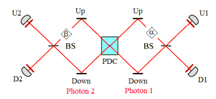
Greenberger, Horne and Zeilinger (GHZ) surveyed the then relatively new field of multiparticle interferometry in their August 1993 Physics Today article, "Multiparticle Interferometry and the Superposition Principle." This tutorial will use Mathcad and tensor algebra to analyze the results associated with their Figure 2, shown below.
Richard Feynman identified the superposition principle, as manifested in the double-slit experiment, as the heart of quantum mechanics and its only mystery. Indeed that simple example of a single-photon superposition illustrates a number of quantum fundamentals, but as GHZ point out multi-photon entangled superpositions reveal additional mysteries like quantum correlations that challenge philosophical positions such as local realism.
The operators required to analyze this two-photon interferometer are defined below. α and β are phase shifters.
Identity:
\[ I = \begin{pmatrix} 1 & 0 \\ 0 & 1 \end{pmatrix} \nonumber \]
Mirror:
\[ M = \begin{pmatrix} 0 & 1 \\ 1 & 0 \end{pmatrix} \nonumber \]
Phase shift:
\[ A ( \delta) = \begin{pmatrix} e^{i \delta} & 0 \\ 0 & 1 \end{pmatrix} \nonumber \]
Beam splitter:
\[ BS = \sqrt{ \frac{1}{2}} \begin{pmatrix} 1 & i \\ i & 1 \end{pmatrix} \nonumber \]
The parametric down converter (PDC) creates two photons traveling in opposite directions in the arms of the interferometer, with photon 1 moving to the right and photon 2 to the left. The initial state is the following entangled superposition.
\[ | \Psi \rangle = \frac{1}{ \sqrt{2}} \left[ | u_1 \rangle |d_2 \rangle + |d_1 \rangle |u_2 \rangle \right] \nonumber \]
\[ | \Psi \rangle = \frac{1}{ \sqrt{2}} \left[ \begin{pmatrix} 1 \\ 0 \end{pmatrix} \otimes \begin{pmatrix} 0 \\ 1 \end{pmatrix} + \begin{pmatrix} 0 \\ 1 \end{pmatrix} \otimes \begin{pmatrix} 1 \\ 0 \end{pmatrix} \right] = \frac{1}{ \sqrt{2}} \left[ \begin{pmatrix} 0 \\ 1 \\ 0 \\ 0 \end{pmatrix} + \begin{pmatrix} 0 \\ 0 \\ 1 \\ 0 \end{pmatrix} \right] = \frac{1}{ \sqrt{2}} \begin{pmatrix} 0 \\ 1 \\ 1 \\ 0 \end{pmatrix} \nonumber \]
There are four output states. The appendix shows how the input and output states are constructed in Mathcad.
\[ | uu \rangle = \begin{pmatrix} 1 \\ 0 \end{pmatrix} \otimes \begin{pmatrix} 1 \\ 0 \end{pmatrix} = \begin{pmatrix} 1 \\ 0 \\ 0 \\ 0 \end{pmatrix} \nonumber \]
\[ | ud \rangle = \begin{pmatrix} 1 \\ 0 \end{pmatrix} \otimes \begin{pmatrix} 0 \\ 1 \end{pmatrix} = \begin{pmatrix} 0 \\ 1 \\ 0 \\ 0 \end{pmatrix} \nonumber \]
\[ | du \rangle = \begin{pmatrix} 0 \\ 1 \end{pmatrix} \otimes \begin{pmatrix} 1 \\ 0 \end{pmatrix} = \begin{pmatrix} 0 \\ 0 \\ 1 \\ 0 \end{pmatrix} \nonumber \]
\[ | dd \rangle = \begin{pmatrix} 0 \\ 1 \end{pmatrix} \otimes \begin{pmatrix} 0 \\ 1 \end{pmatrix} = \begin{pmatrix} 0 \\ 0 \\ 0 \\ 1 \end{pmatrix} \nonumber \]
The input and output states are defined in Mathcad syntax.
\[ u = \begin{pmatrix} 1 \\ 0 \end{pmatrix} \nonumber \]
\[ d = \begin{pmatrix} 0 \\ 1 \end{pmatrix} \nonumber \]
\[ \Psi = \frac{1}{ \sqrt{2}} \begin{pmatrix} 0 \\ 1 \\ 1 \\ 0 \end{pmatrix} \nonumber \]
\[ u1u2 = \begin{pmatrix} 1 \\ 0 \\ 0 \\ 0 \end{pmatrix} \nonumber \]
\[ u1d2 = \begin{pmatrix} 0 \\ 1 \\ 0 \\ 0 \end{pmatrix} \nonumber \]
\[ d1u2 = \begin{pmatrix} 0 \\ 0 \\ 1 \\ 0 \end{pmatrix} \nonumber \]
\[ d1d2 = \begin{pmatrix} 0 \\ 0 \\ 0 \\ 1 \end{pmatrix} \nonumber \]
The four outcome probabilities are now calculated. The appendix shows how Mathcad is used to carry out the tensor product of two matrices.
\[ P{u1u2} ( \alpha , \beta ) = \left( \left| u1u2^T \text{kronecker} (BS,~BS) \text{kronecker} (A ( \alpha), A ( \beta )) \text{kronecker} (M,~M) \Psi \right| \right)^2 \nonumber \]
\[ P{u1d2} ( \alpha , \beta ) = \left( \left| u1d2^T \text{kronecker} (BS,~BS) \text{kronecker} (A ( \alpha), A ( \beta )) \text{kronecker} (M,~M) \Psi \right| \right)^2 \nonumber \]
\[ P{d1u2} ( \alpha , \beta ) = \left( \left| d1u2^T \text{kronecker} (BS,~BS) \text{kronecker} (A ( \alpha), A ( \beta )) \text{kronecker} (M,~M) \Psi \right| \right)^2 \nonumber \]
\[ P{d1d2} ( \alpha , \beta ) = \left( \left| d1d2^T \text{kronecker} (BS,~BS) \text{kronecker} (A ( \alpha), A ( \beta )) \text{kronecker} (M,~M) \Psi \right| \right)^2 \nonumber \]
The probability that the individual detectors will fire is given by the following sums.
\[ P_{u1} = P_{u1u2} + P_{u1d2} \nonumber \]
\[ P_{d1} = P_{d1d2} + P_{d1u2} \nonumber \]
\[ P_{u2} = P_{u1u2} + P_{d1u2} \nonumber \]
\[ P_{d2} = P_{d1d2} + P_{u1d2} \nonumber \]
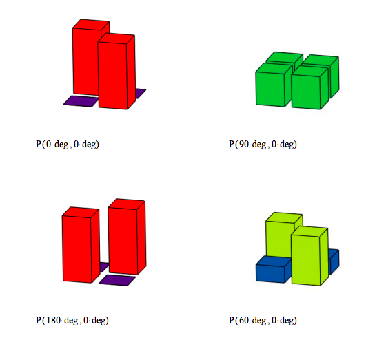
Because only the phase difference between the two arms of the interferometer matters, β is set to zero and the phase difference is expressed in the value of α. The following graphs show the behavior of the detector pairings as a function of the phase difference α.
\( \alpha = 0 \text{deg}, 1 \text{deg} .. 360 \text{deg}\)
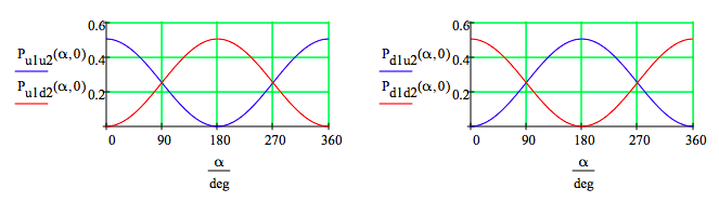
When there is no phase difference in the two branches of the interferometer there is a strong correlation in the detector responses. Fifty percent of the time the photons arrive at the up-detectors and 50% of the time at the down-detectors. There are no coincidences between an up and a down detector. This might be called bosonic behavior - bosons like to do the same thing.
For convenience results will also be presented in numeric format. See the Appendix for a graphical display.
\( \alpha = 0 ~ \text{deg}\)
\[ \begin{pmatrix} P_{u1u2} ( \alpha ,0) & P_{u1d2} ( \alpha ,0) \\ P_{d1u2} ( \alpha ,0) & P_{d1d2} ( \alpha ,0) \end{pmatrix} = \begin{pmatrix} 0.5 & 0 \\ 0 & 0.5 \end{pmatrix} \nonumber \]
A 90 degree phase difference results in no correlation. The four detector pairs fire with equal frequency.
\( \alpha = 90 ~ \text{deg}\)
\[ \begin{pmatrix} P_{u1u2} ( \alpha ,0) & P_{u1d2} ( \alpha ,0) \\ P_{d1u2} ( \alpha ,0) & P_{d1d2} ( \alpha ,0) \end{pmatrix} = \begin{pmatrix} 0.25 & 0.25 \\ 0.25 & 0.25 \end{pmatrix} \nonumber \]
A 180 degree phase difference results in what might be called fermionic behavior. If one photon is detected at an up-detector, the other is registered at a down detector. They never both arrive at the same type of detector. Fermions don't like to do the same thing at the same time.
\( \alpha = 180 ~ \text{deg}\)
\[ \begin{pmatrix} P_{u1u2} ( \alpha ,0) & P_{u1d2} ( \alpha ,0) \\ P_{d1u2} ( \alpha ,0) & P_{d1d2} ( \alpha ,0) \end{pmatrix} = \begin{pmatrix} 0 & 0.5 \\ 0.5 & 0 \end{pmatrix} \nonumber \]
Intermediate correlation is achieved with a 60 degree phase difference.
\( \alpha = 60 ~ \text{deg}\)
\[ \begin{pmatrix} P_{u1u2} ( \alpha ,0) & P_{u1d2} ( \alpha ,0) \\ P_{d1u2} ( \alpha ,0) & P_{d1d2} ( \alpha ,0) \end{pmatrix} = \begin{pmatrix} 0.375 & 0.125 \\ 0.125 & 0.375 \end{pmatrix} \nonumber \]
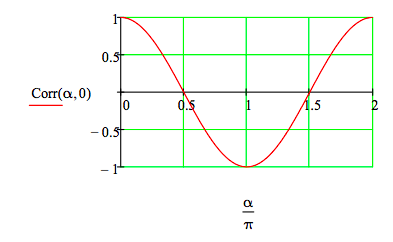
These tabular results can be summarized by displaying the correlation function. Perfect correlation +1; perfect anti-correlation -1; no correlation 0. Another graphical display can be found in the Appendix.
\( \alpha = 0, .02 .. 2 \pi \)
\[ \text{Corr} ( \alpha , \beta ) = P_{u1u2} ( \alpha , \beta ) - P_{u1d2} ( \alpha , \beta ) - P_{d1u2} ( \alpha , \beta ) + P_{d1d2} ( \alpha , \beta ) \nonumber \]
Note that the sums of the rows and the sums of the columns in the tables above always equal 1/2.
\[ P_{1u} = P_{2u} = P_{1d} = P_{2d} = \frac{1}{2} \nonumber \]
An individual detector fires 50% of the time in spite of the correlations that may occur between two detectors. Looking at individual detectors locally reveals totally random behavior. It is only when coincidences between pairs of detectors on the left and right are examined that correlations are observed.
The random behavior at each of the detectors can be directly shown by calculations in which only one detector is being monitored. This requires the projection operators for up and down motion given below. The calculations are shown for the arbitrary phases shown below. However, all phase relationships give the same results.
Projection operators:
\[ uu^T = \begin{pmatrix} 1 & 0 \\ 0 & 0 \end{pmatrix} ~~~ dd^T = \begin{pmatrix} 0 & 0 \\ 0 & 1 \end{pmatrix} \nonumber \]
Phases:
\[ \alpha = 11~ \text{deg} ~~~ \beta = 58 ~ \text{deg} \nonumber \]
\[ \begin{array}{r}
Detector & Probability of Firing \\
U1 & \left( \left| \left( uu^T , ~I \right) \text{kronecker} (BS,~BS) \text{kronecker} (A ( \alpha), A ( \beta )) \text{kronecker} (M,~M) \Psi \right| \right)^2 = 0.5 \\
D1 & \left( \left| \left( dd^T , ~I \right) \text{kronecker} (BS,~BS) \text{kronecker} (A ( \alpha), A ( \beta )) \text{kronecker} (M,~M) \Psi \right| \right)^2 = 0.5 \\
U2 & \left( \left| \left( I, ~ uu^T \right) \text{kronecker} (BS,~BS) \text{kronecker} (A ( \alpha), A ( \beta )) \text{kronecker} (M,~M) \Psi \right| \right)^2 = 0.5 \\
D2 & \left( \left| \left( I,~ dd^T \right) \text{kronecker} (BS,~BS) \text{kronecker} (A ( \alpha), A ( \beta )) \text{kronecker} (M,~M) \Psi \right| \right)^2 = 0.5 \\
\end{array} \nonumber \]
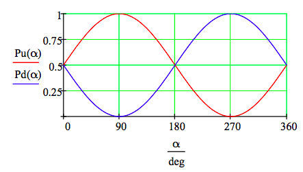
At this point it is important to recall that interference at the individual detectors would be observed if the photons were not entangled. Looking at either half of the interferometer shown above and assuming an unentangled photon in the superposition, \( \frac{1}{ \sqrt{2}} \begin{pmatrix} 1 \\ 1 \end{pmatrix}\), of being in the upper and lower arms of the truncated interferometer results in interference effects as a function of α at the detectors as is illustrated in the following graph.
\( \alpha = 0 ~ \text{deg}, 1~ \text{deg} .. 360 ~ \text{deg}\)
\[ Pu ( \alpha ) = \left[ \left| uu^T BS A ( \alpha ) M \frac{1}{ \sqrt{2}} \begin{pmatrix} 1 \\ 1 \end{pmatrix} \right| \right]^2 \nonumber \]
\[ Pd ( \alpha ) = \left[ \left| dd^T BS A ( \alpha ) M \frac{1}{ \sqrt{2}} \begin{pmatrix} 1 \\ 1 \end{pmatrix} \right| \right]^2 \nonumber \]
Recently, Art Hobson posted "Implications of bipartite interferometry for the measurement problem" at arXiv:1301.1673. In this manuscript he deals in depth with the results presented above. Therefore, in concluding this tutorial I will take relevant commentary from his manuscript without further comment. However, some excerpts have been slightly modified, but not in such a way as to change their original meanings.
- When two photons are entangled, the state actually detected by an observer of either photon is the local or reduced state of that photon. The reduced state operator of photon 2 is obtained by averaging (tracing) the total density operator over photon 1 as is shown below. This procedure shows that photon 2's reduced or local state operator is diagonal indicating a classical mixed state - it has been stripped of its off-diagonal interference terms. This result is consistent with the random behavior noted earlier for the measurements on individual photons.
\[ \hat{ \rho}_{12} = | \Psi \rangle \langle \Psi | = \frac{1}{2} [ |u_1 \rangle |d_2 \rangle \langle d_2 | \langle u_1 | + | u_1 \rangle |d_2 \rangle \langle u_2 | \langle d_1 | + | d_1 \rangle |u_2 \rangle \langle d_2 | \langle u_1 | + | d_1 \rangle | u_2 \rangle \langle u_2 | \rangle d_1 |] \nonumber \]
\[ \hat{ \rho}_2 = \frac{1}{2} [ \langle u_1 | \Psi \rangle \langle \Psi | u_1 \rangle + \langle d_1 | \Psi \rangle \langle \Psi | d_1 \rangle ] = \frac{1}{2} [ |d_2 \rangle \langle d_2 | + | u_2 \rangle \langle u_2 |] \nonumber \]
- Therefore, when a bipartite system is in an entangled superposition, its subsystems are not in superpositions but are instead mixed states with each subsystem in a definite, but unknown state.
- The detectors (U1, D1, U2, D2) show no local signs of interference of the type that would occur if the photons were not entangled, because each photon is a "which path" detector for the other photon, decohering the other photon and creating incoherent local mixtures.
- To summarize, an entangled photon is always "in" its local state, the state described by its reduced density operator (see above), because this is the state actually detected by an observer of the photon. The entangled state Ψ is a global superposition of photon correlations, not a superposition of local photon states.
Appendix
The tensor product of two vectors is shown below.
\[ \begin{pmatrix} a \\ b \end{pmatrix} \otimes \begin{pmatrix} c \\ d \end{pmatrix} = \begin{pmatrix} ac \\ ad \\ bc \\ bd \end{pmatrix} \nonumber \]
Mathcad does not have a command for the vector tensor product, so it is necessary to develop a way of implementing it using kronecker, which requires square matrices. For this reason the spin vector is stored in the left column of a 2x2 matrix by augmenting the spin vector with the null vector. After the matrix tensor products have been carried out using kronecker the final spin vector resides in the left column of the final square matrix. Next the submatrix command is used to save this column, discarding the rest of the matrix.
The Mathcad syntax for the tensor multiplication of two vectors is as follows.
\[ \Psi ( a,~b) = \text{submatrix} \left[ \text{kronecker} \left[ \text{augment} \left[ a, ~ \begin{pmatrix} 0 \\ 0 \end{pmatrix} \right] , \text{augment} \left[ b,~ \begin{pmatrix} 0 \\ 0 \end{pmatrix} \right] \right] , ~1,~4,~1,~1 \right] \nonumber \]
The initial photon state:
\[ \frac{1}{ \sqrt{2}} ( \Psi (u,~d) + \Psi (d,~u)) = \begin{pmatrix} 0 \\ 0.707 \\ 0.707 \\ 0 \end{pmatrix} \nonumber \]
Tensor matrix multiplication is also known as Kronecker multiplication. Here it is shown that the Mathcad result using the kronecker command is identical to the hand calculation.
\[ \text{kronecker} (BS,~BS) = \begin{pmatrix} 0.5 & 0.5i & 0.5i & -0.5i \\ 0.5i & 0.5 & -0.5 & 0.5i \\ 0.5i & -0.5 & 0.5 & 0.5i \\ -0.5 & 0.5i & 0.5i & 0.5 \end{pmatrix} \nonumber \]
\[ \widehat{BS} \otimes \widehat{BS} = \frac{1}{ \sqrt{2}} \begin{pmatrix} 1 & i \\ i & 1 \end{pmatrix} \otimes \frac{1}{ \sqrt{2}} \begin{pmatrix} 1 & i \\ i & 1 \end{pmatrix} = \frac{1}{2} \begin{pmatrix} 1 \begin{pmatrix} 1 & i \\ i & 1 \end{pmatrix} & i \begin{pmatrix} 1 & i \\ i & 1 \end{pmatrix} \\ i \begin{pmatrix} 1 & i \\ i & 1 \end{pmatrix} & 1 \begin{pmatrix} 1 & i \\ i & 1 \end{pmatrix} \end{pmatrix} = \frac{1}{2} \begin{pmatrix} 1 & i & i & -1 \\ i & 1 & -1 & i \\ i & -1 & 1 & i \\ -1 & i & i & 1 \end{pmatrix} \nonumber \]
A graphical display of tabular results presented earlier:
\[ P ( \alpha , \beta ) = \begin{pmatrix} P_{u1u2} ( \alpha , \beta ) & P_{u1d2} ( \alpha , \beta ) \\ P_{d1u2} ( \alpha , \beta ) & P_{d1d2} ( \alpha , \beta ) \end{pmatrix} \nonumber \]
The following algebraic analysis of the experiment shows the evolution of the original entangled state. Consistent with the matrix mechanics analysis, it shows that when the phase diference is zero both photons arrive at either the U- or the D-detectors, and when the phase difference is π one photon arrives at U-detector and the other at the D-detector.
\( \alpha = 0 ~~~ \beta = 0\)
\[ \frac{1}{ \sqrt{2}} (u_1 d_2 + d_1 u_2)~ \begin{array}{|l}
\text{substitute},~ u1 = \frac{e^{i \alpha}}{ \sqrt{2}} (i U1 + D1) \\
\text{substitute},~ d2 = \frac{1}{ \sqrt{2}} (U2 + iD2) \\
\text{substitute},~ u1 = \frac{1}{ \sqrt{2}} (U1 + D1) \\
\text{substitute},~ d2 = \frac{e^{i \beta}}{ \sqrt{2}} (i U2 + D2) \\
\end{array} \rightarrow \sqrt{2} \left( \frac{U1 U2 i}{2} + \frac{D1 D2 i}{2} \right) \nonumber \]
\( \alpha = \pi ~~~ \beta = 0\)
\[ \frac{1}{ \sqrt{2}} (u_1 d_2 + d_1 u_2)~ \begin{array}{|l}
\text{substitute},~ u1 = \frac{e^{i \alpha}}{ \sqrt{2}} (i U1 + D1) \\
\text{substitute},~ d2 = \frac{1}{ \sqrt{2}} (U2 + iD2) \\
\text{substitute},~ u1 = \frac{1}{ \sqrt{2}} (U1 + D1) \\
\text{substitute},~ d2 = \frac{e^{i \beta}}{ \sqrt{2}} (i U2 + D2) \\
\end{array} \rightarrow \sqrt{2} \left( \frac{D1 U2}{2} - \frac{D2 U2}{2} \right) \nonumber \]