7.29: Two-photon Interferometry

Last updated
Save as PDF

Page ID: 142146

\( \newcommand{\vecs}[1]{\overset { \scriptstyle \rightharpoonup} {\mathbf{#1}} } \) \( \newcommand{\vecd}[1]{\overset{-\!-\!\rightharpoonup}{\vphantom{a}\smash {#1}}} \)\(\newcommand{\id}{\mathrm{id}}\) \( \newcommand{\Span}{\mathrm{span}}\) \( \newcommand{\kernel}{\mathrm{null}\,}\) \( \newcommand{\range}{\mathrm{range}\,}\) \( \newcommand{\RealPart}{\mathrm{Re}}\) \( \newcommand{\ImaginaryPart}{\mathrm{Im}}\) \( \newcommand{\Argument}{\mathrm{Arg}}\) \( \newcommand{\norm}[1]{\| #1 \|}\) \( \newcommand{\inner}[2]{\langle #1, #2 \rangle}\) \( \newcommand{\Span}{\mathrm{span}}\) \(\newcommand{\id}{\mathrm{id}}\) \( \newcommand{\Span}{\mathrm{span}}\) \( \newcommand{\kernel}{\mathrm{null}\,}\) \( \newcommand{\range}{\mathrm{range}\,}\) \( \newcommand{\RealPart}{\mathrm{Re}}\) \( \newcommand{\ImaginaryPart}{\mathrm{Im}}\) \( \newcommand{\Argument}{\mathrm{Arg}}\) \( \newcommand{\norm}[1]{\| #1 \|}\) \( \newcommand{\inner}[2]{\langle #1, #2 \rangle}\) \( \newcommand{\Span}{\mathrm{span}}\)\(\newcommand{\AA}{\unicode[.8,0]{x212B}}\)

In this experiment a parametric down converter, PDC, transforms an incident photon into two lower energy photons, one horizontally polarized and the other vertically polarized. One photon takes the upper path and the other the lower path or vice versa. The upper branch of the apparatus contains a polarization rotator, θ. The photon paths are combined at a 50-50 beam splitter, after which they interact with a polarizing beam splitter which separates horizontal (transmitted) and vertical (reflected) polarization. The results of this experiment are that no matter the angle θ both photons are detected at either the upper set of detectors (uh,dv) or the lower set of detectors (uv,dh). One photon is never detected at the upper set of detectors while the other is detected at the lower set of detectors. A quantum mechanical analysis of this phenomena is provided below.

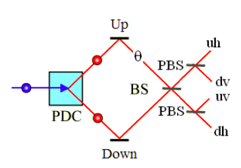
Screen Shot 2019-03-04 at 12.12.11 PM.png

PDC = Parametric Down Converter

BS = Beam Splitter

PBS = Polarizing Beam Splitter

uh = moving up, horizontal polarization

dv = moving down, vertical polarization

uv = moving up, vertical polarization

dh = moving down, horizontal polarization

θ = polarization rotator

The vectors representing the motional and polarization states of the photons are:

Motional states:

\[ u = \begin{pmatrix} 1 \\ 0 \end{pmatrix} \nonumber \]

\[ d = \begin{pmatrix} 0 \\ 1 \end{pmatrix} \nonumber \]

Polarization states:

\[ h = \begin{pmatrix} 1 \\ 0 \end{pmatrix} \nonumber \]

\[ v = \begin{pmatrix} 0 \\ 1 \end{pmatrix} \nonumber \]

There are four motional-polarization photon states after the PDC. These are formed by the tensor product of the appropriate motional and polarization vectors.

Combined motional and polarization states:

\[ uh = \begin{pmatrix} 1 \\ 0 \\ 0 \\ 0 \end{pmatrix} \nonumber \]

\[ uv = \begin{pmatrix} 0 \\ 1 \\ 0 \\ 0 \end{pmatrix} \nonumber \]

\[ dh = \begin{pmatrix} 0 \\ 0 \\ 1 \\ 0 \end{pmatrix} \nonumber \]

\[ dv = \begin{pmatrix} 0 \\ 0 \\ 0 \\ 1 \end{pmatrix} \nonumber \]

The optical devices are represented by matrices and operate on the vector states of the photons.

Rotation:

\[ R( \theta ) \begin{pmatrix} \cos \theta & - \sin \theta \\ \sin \theta & \cos \theta \end{pmatrix} \nonumber \]

Beam splitter:

\[ BS = \frac{1}{ \sqrt{2}} \begin{pmatrix} 1 & i \\ i & 1 \end{pmatrix} \nonumber \]

Polarizing beam splitter:

\[ PBS = \begin{pmatrix} 1 & 0 & 0 & 0 \\ 0 & 0 & 0 & 1 \\ 0 & 0 & 1 & 0 \\ 0 & 1 & 0 & 0 \end{pmatrix} \nonumber \]

An operator for the mirrors is not necessary, because if it is included it has no effect on the measurement results. The identity and a null matrix are also required as will be seen below.

Identity:

\[ I = \begin{pmatrix} 1 & 0 \\ 0 & 1 \end{pmatrix} \nonumber \]

Null matrix:

\[ N = \begin{pmatrix} 0 & 0 & 0 \\ 0 & 0 & 0 \\ 0 & 0 & 0 \\ 0 & 0 & 0 \end{pmatrix} \nonumber \]

The photon state after the PDC is a even superposition of all possible motional-polarization states.

\[ | \Psi \rangle _i = \frac{1}{2} [ |uh \rangle |dv \rangle + |uv \rangle |dh \rangle + |dh \rangle |uv \rangle + |dv \rangle |uh \rangle ] = \frac{1}{2} \left[ \begin{pmatrix} 1 \\ 0 \\ 0 \\ 0 \end{pmatrix} \otimes \begin{pmatrix} 0 \\ 0 \\ 0 \\ 1 \end{pmatrix} + \begin{pmatrix} 0 \\ 1 \\ 0 \\ 0 \end{pmatrix} \otimes \begin{pmatrix} 0 \\ 0 \\ 1 \\ 0 \end{pmatrix} + \begin{pmatrix} 0 \\ 0 \\ 1 \\ 0 \end{pmatrix} \otimes \begin{pmatrix} 0 \\ 1 \\ 0 \\ 0 \end{pmatrix} + \begin{pmatrix} 0 \\ 0 \\ 0 \\ 1 \end{pmatrix} \otimes \begin{pmatrix} 1 \\ 0 \\ 0 \\ 0 \end{pmatrix} \right] \nonumber \]

This state is formed as follows using Mathcad's kronecker command.

\[ \Psi (a, b) = \text{submatrix} [ \text{kronecker} [ \text{augment} (a, N),~ ( \text{augment}(b, N)), 1,~16,~1,~1] \nonumber \]

\[ \Psi_i = \frac{1}{2} \left( \Psi_{(uh,~dv)} + \Psi_{(uv,~dvh)} + \Psi_{(dh,~uv)} + \Psi_{(dv,~uh)} \right) \nonumber \]

\[ \Psi_i^T = \begin{pmatrix} 0 & 0 & 0 & 0.5 & 0 & 0 & 0.5 & 0 & 0 & 0.5 & 0 & 0 & 0.5 & 0 & 0 & 0 \end{pmatrix} \nonumber \]

The final state is calculated as a function of the orientation of the polarization rotator.

\[ \Psi_f ( \theta) = \text{kronecker} (PBS,PBS) \text{kronecker} (BS, \text{kronecker} (I, \text{kronecker} (BS,~ I))) \text{kronecker} (I,~ \text{kronecker} (R, ( \theta), \text{kronecker} (I,~ I))) \Psi_i \nonumber \]

For θ = 0 the detected states are |uh>|dv>, |uv>|dh>, |dh>|uv> and |dv>|uh> each with a 25% probability of occurrence.

\[ \begin{bmatrix} \left( \left| \Psi (uh, uh) \Psi_f ( \theta) \right| \right)^2 & \left( \left| \Psi (uh, uv) \Psi_f ( \theta) \right| \right)^2 & \left( \left| \Psi (uh, dh) \Psi_f ( \theta) \right| \right)^2 & \left( \left| \Psi (uh, dv) \Psi_f ( \theta) \right| \right)^2 \\ \left( \left| \Psi (uv, uh) \Psi_f ( \theta) \right| \right)^2 & \left( \left| \Psi (uv, uv) \Psi_f ( \theta) \right| \right)^2 & \left( \left| \Psi (uv, dh) \Psi_f ( \theta) \right| \right)^2 & \left( \left| \Psi (uv, dv) \Psi_f ( \theta) \right| \right)^2 \\ \left( \left| \Psi (dh, uh) \Psi_f ( \theta) \right| \right)^2 & \left( \left| \Psi (dh, uv) \Psi_f ( \theta) \right| \right)^2 & \left( \left| \Psi (dh, dh) \Psi_f ( \theta) \right| \right)^2 & \left( \left| \Psi (dh, dv) \Psi_f ( \theta) \right| \right)^2 \\ \left( \left| \Psi (dv, uh) \Psi_f ( \theta) \right| \right)^2 & \left( \left| \Psi (dv, uv) \Psi_f ( \theta) \right| \right)^2 & \left( \left| \Psi (dv, dh) \Psi_f ( \theta) \right| \right)^2 & \left( \left| \Psi (dv, dv) \Psi_f ( \theta) \right| \right)^2 \end{bmatrix} = \begin{pmatrix} 0 & 0 & 0 & \frac{1}{4} \\ 0 & 0 & \frac{1}{4} & 0 \\ 0 & \frac{1}{4} & 0 & 0 \\ \frac{1}{4} & 0 & 0 & 0 \end{pmatrix} \nonumber \]

For \( \theta = \frac{ \pi}{2}\) the detected states are |uh>|uh>, |uv>|uv>, |dh>|dh> and |dv>|dv> each with a 25% probability of occurrence.

\[ \begin{bmatrix} \left( \left| \Psi (uh, uh) \Psi_f ( \theta) \right| \right)^2 & \left( \left| \Psi (uh, uv) \Psi_f ( \theta) \right| \right)^2 & \left( \left| \Psi (uh, dh) \Psi_f ( \theta) \right| \right)^2 & \left( \left| \Psi (uh, dv) \Psi_f ( \theta) \right| \right)^2 \\ \left( \left| \Psi (uv, uh) \Psi_f ( \theta) \right| \right)^2 & \left( \left| \Psi (uv, uv) \Psi_f ( \theta) \right| \right)^2 & \left( \left| \Psi (uv, dh) \Psi_f ( \theta) \right| \right)^2 & \left( \left| \Psi (uv, dv) \Psi_f ( \theta) \right| \right)^2 \\ \left( \left| \Psi (dh, uh) \Psi_f ( \theta) \right| \right)^2 & \left( \left| \Psi (dh, uv) \Psi_f ( \theta) \right| \right)^2 & \left( \left| \Psi (dh, dh) \Psi_f ( \theta) \right| \right)^2 & \left( \left| \Psi (dh, dv) \Psi_f ( \theta) \right| \right)^2 \\ \left( \left| \Psi (dv, uh) \Psi_f ( \theta) \right| \right)^2 & \left( \left| \Psi (dv, uv) \Psi_f ( \theta) \right| \right)^2 & \left( \left| \Psi (dv, dh) \Psi_f ( \theta) \right| \right)^2 & \left( \left| \Psi (dv, dv) \Psi_f ( \theta) \right| \right)^2 \end{bmatrix} = \begin{pmatrix} \frac{1}{4} & 0 & 0 & 0 \\ 0 & \frac{1}{4} & 0 & 0 \\ 0 & 0 & \frac{1}{4} & 0 \\ 0 & 0 & 0 & \frac{1}{4} \end{pmatrix} \nonumber \]

For \( \theta = \frac{ \pi}{4}\) the results of the previous examples occur with each state being observed with a probability of 12.5%.

\[ \begin{bmatrix} \left( \left| \Psi (uh, uh) \Psi_f ( \theta) \right| \right)^2 & \left( \left| \Psi (uh, uv) \Psi_f ( \theta) \right| \right)^2 & \left( \left| \Psi (uh, dh) \Psi_f ( \theta) \right| \right)^2 & \left( \left| \Psi (uh, dv) \Psi_f ( \theta) \right| \right)^2 \\ \left( \left| \Psi (uv, uh) \Psi_f ( \theta) \right| \right)^2 & \left( \left| \Psi (uv, uv) \Psi_f ( \theta) \right| \right)^2 & \left( \left| \Psi (uv, dh) \Psi_f ( \theta) \right| \right)^2 & \left( \left| \Psi (uv, dv) \Psi_f ( \theta) \right| \right)^2 \\ \left( \left| \Psi (dh, uh) \Psi_f ( \theta) \right| \right)^2 & \left( \left| \Psi (dh, uv) \Psi_f ( \theta) \right| \right)^2 & \left( \left| \Psi (dh, dh) \Psi_f ( \theta) \right| \right)^2 & \left( \left| \Psi (dh, dv) \Psi_f ( \theta) \right| \right)^2 \\ \left( \left| \Psi (dv, uh) \Psi_f ( \theta) \right| \right)^2 & \left( \left| \Psi (dv, uv) \Psi_f ( \theta) \right| \right)^2 & \left( \left| \Psi (dv, dh) \Psi_f ( \theta) \right| \right)^2 & \left( \left| \Psi (dv, dv) \Psi_f ( \theta) \right| \right)^2 \end{bmatrix} = \begin{pmatrix} \frac{1}{8} & 0 & 0 & \frac{1}{0} \\ 0 & \frac{1}{8} & \frac{1}{8} & 0 \\ 0 & \frac{1}{8} & \frac{1}{8} & 0 \\ \frac{1}{8} & 0 & 0 & \frac{1}{8} \end{pmatrix} \nonumber \]