7.21: Two Analyses of the Michelson Interferometer
- Page ID
- 141687

Path difference between interferometer arms is δ. Phase accumulated due to path difference: \( exp \left( i \frac{2 \pi \delta}{ \lambda} \right) \)
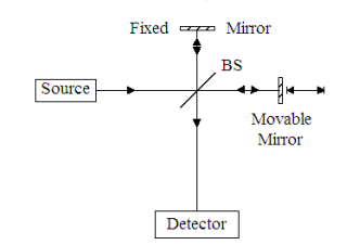
S stands for source, D for detector, T for transmitted and R for reflected. The evolution of the photon wave function at various stages is given below.
\[ S = \frac{1}{ \sqrt{2}} (T + iR) \nonumber \]
\[ T = \frac{ exp \left( i \frac{2 \pi \delta}{ \lambda} \right)}{ \sqrt{2}} (iD + S) \nonumber \]
\[ R = \frac{1}{ \sqrt{2}} (D + iS) \nonumber \]
\[ S = \frac{1}{ \sqrt{2}} (T +iR) |^{substitute,~T = \frac{exp \left( i \frac{2 \pi \delta}{ \lambda}\right)}{ \sqrt{2}} (iD+S)}_{substitute,~R = \frac{1}{ \sqrt{2}} (D + iS)} \rightarrow S = - \frac{S}{2} + \frac{S e^{ \frac{2i \pi \delta}{ \lambda}}}{2} + \frac{D e^{ \frac{2i \pi \delta}{ \lambda}}}{2} + \frac{Di}{2} \nonumber \]
The probability the photon will arrive at the detector is the square of the absolute magnitude of the coefficient of D.
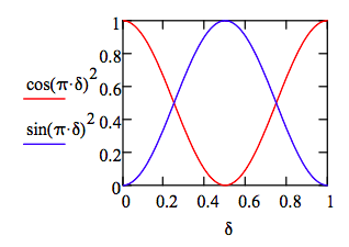
\[ \frac{-1}{2} \left( e^{ \frac{-2 i \pi \delta}{ \lambda}} \right) \frac{1}{2} \left( e^{ \frac{-2 i \pi \delta}{ \lambda}} \right) simplify~ \rightarrow \sin \left( \frac{ \pi \delta}{ \lambda} \right)^2 \nonumber \]
The same results are now illustrated using a matrix mechanics approach. Horizontal and vertical motion of the photon are represented by vectors. The source emits a horizontal photon, the detector receives a vertical photon. The beam splitter and the phase shift due to path length difference are represented by matrices. A matrix representation for the mirrors is unnecessary because the simply return the photon to the beam splitter.
Horizontal motion: \( \begin{pmatrix} 1 \\ 0 \end{pmatrix}\)
Vertical motion: \( \begin{pmatrix} 0 \\ 1 \end{pmatrix}\)
Beam splitter:
\[ BS = \begin{pmatrix} \frac{1}{ \sqrt{2}} & \frac{1}{ \sqrt{2}} \\ \frac{1}{ \sqrt{2}} & \frac{1}{ \sqrt{2}} \end{pmatrix} \nonumber \]
Phase shift:
\[ A ( \delta) = \begin{pmatrix} e^{2 i \pi \frac{ \delta}{ \lambda}} & 0 \\ 0 & 1 \end{pmatrix} \nonumber \]
Calculate the probability amplitude and probability that the photon will arrive at the detector
\[ \begin{pmatrix} 0 & 1 \end{pmatrix} BS \begin{pmatrix} e^{2 i \pi \frac{ \delta}{ \lambda}} & 0 \\ 0 & 1 \end{pmatrix} BS \begin{pmatrix} 1 \\ 0 \end{pmatrix} \rightarrow \frac{e^{ \frac{2i \pi \delta}{ \lambda}}}{2} + \frac{1}{2} i \nonumber \]
\[ \left( \frac{e^{ \frac{-2i \pi \delta}{ \lambda} (-i)}}{2} + \frac{1}{2} (-i) \right) \left( \frac{e^{ \frac{2i \pi \delta}{ \lambda} (i)}}{2} + \frac{1}{2} i \right) simplify \rightarrow \cos \left( \frac{\pi \delta}{ \lambda}\right)^2 \nonumber \]
Calculate the probability amplitude and probability that the photon will be returned to the source.
\[ \begin{pmatrix} 1 & 0 \end{pmatrix} BS \begin{pmatrix} e^{2i \pi \frac{ \delta}{ \lambda}} & 0 \\ 0 & 1 \end{pmatrix} BS \begin{pmatrix} 1 \\ 0 \end{pmatrix} \rightarrow \frac{e ^{ \frac{2 i \pi \delta}{ \lambda}}}{2} - \frac{1}{2} \nonumber \]
\[ \left( \frac{e^{ \frac{-2i \pi \delta}{ \lambda}}}{2} - \frac{1}{2} \right) \left( \frac{e^{ \frac{2i \pi \delta}{ \lambda}}}{2} - \frac{1}{2} \right) simplify \rightarrow \sin \left( \frac{\pi \delta}{ \lambda}\right)^2 \nonumber \]
Plotting these results in units of λ yields:
\[ \delta = 0, .01 .. 1 \nonumber \]