1.97: Quantum Dynamics- One Step at a Time

Integration of the time‐dependent Schrödinger equation

\[
i \hbar \frac{d|\Psi(t)\rangle}{d t}=H(\hat{p}, \hat{x})|\Psi(t)\rangle
\nonumber \]

yields

\[
|\Psi(t+\tau)\rangle=\exp \left(\frac{-i H(\hat{p}, \hat{x}) \tau}{\hbar}\right)|\Psi(t)\rangle=\exp \left(\frac{-i T(\hat{p}) \tau}{\hbar}\right) \exp \left(\frac{-i V(\hat{x}) \tau}{\hbar}\right)|\Psi(t)\rangle
\nonumber \]

The purpose of this tutorial is to show how this single time‐step calculation is implemented. In the above equation, T (\(\hat{p}\)) and V (\(\hat{x}\)) are the kinetic and potential energy operators, and τ is the time increment. However, it is not immediately obvious how the exponential time‐evolution operator operates on the wave function. For example, in the coordinate representation \(\hat{x}\) is a multiplicative operator, but \(\hat{p}\) is a differential operator (see any introductory quantum or physical chemistry textbook).

The tactic that will be employed is to carry out the potential energy operation in coordinate space where the position operator is multiplicative and Fourier transform the result to momentum space where the momentum operator is multiplicative. After operation by the kinetic energy operator the result is Fourier transformed back to coordinate space and displayed.

This procedure requires the following mathematical tools.

The coordinate‐space eigenvalue equation and completeness relation:

\[
\hat{x}|x\rangle=|x\rangle x \qquad \int|x\rangle\langle x| d x=1
\nonumber \]

The momentum‐space eigenvalue equation and completeness relation:

\[
\hat{p}|p\rangle=|p\rangle p \qquad \int|p\rangle\langle p| d p=1
\nonumber \]

The Fourier transforms between position and momentum:

\[
\langle x | p\rangle=\langle p | x\rangle^{*}=\frac{1}{\sqrt{2 \pi}} \exp \left(\frac{i p x}{\hbar}\right)
\nonumber \]

With these preliminaries out of the way the first step is to insert the coordinate completeness relation between the exponential potential energy operator and the wave function. In other words, we are going to work initially in coordinate space.

\[
|\Psi(t+\tau)\rangle=\int \exp \left(\frac{-i T(\hat{p}) \tau}{\hbar}\right) \exp \left(\frac{-i V(\hat{x}) \tau}{\hbar}\right)|x|\langle x | \Psi(t)\rangle d x
\nonumber \]

The next step is to carry out a series expansion on the potential energy operator. To see what happens we will assume, for the sake of mathematical clarity, the potential energy operator is simply \(\hat{x}\). Here we make use of the coordinate space eigenvalue equation to take the “hat” off the position operator.

\[
\exp \left(-\frac{i \hat{x} \tau}{\hbar}\right)|x\rangle=\left(1-\frac{i \hat{x} \tau}{\hbar}-\frac{\hat{x}^{2} \tau^{2}}{2 \hbar^{2}}+\cdots\right)|x\rangle=|x\rangle\left(1-\frac{i x \tau}{\hbar}-\frac{x^{2} \tau^{2}}{2 \hbar^{2}}+\cdots\right)=|x\rangle \exp \left(-\frac{i x \tau}{\hbar}\right)
\nonumber \]

In general, for an operator operating in its “eigen space” we have,

\[
\exp \left(-\frac{i \hat{\delta} \tau}{\hbar}\right)|o\rangle=|o\rangle \exp \left(-\frac{i o \tau}{\hbar}\right)
\nonumber \]

The first two steps have brought us to this point.

\[
|\Psi(t+\tau)\rangle=\int \exp \left(\frac{-i T(\hat{p}) \tau}{\hbar}\right)|x\rangle \exp \left(\frac{-i V(x) \tau}{\hbar}\right)\langle x | \Psi(t)\rangle d x
\nonumber \]

Now we Fourier transform to momentum space by inserting the momentum completeness relation between the exponential kinetic energy operator and \(|x\rangle \).

\[
|\Psi(t+\tau)\rangle=\iint \exp \left(\frac{-i T(\hat{p}) \tau}{\hbar}\right)|p\rangle\langle p | x\rangle \exp \left(\frac{-i V(x) \tau}{\hbar}\right)\langle x | \Psi(t)\rangle d x d p
\nonumber \]

The procedure used for the potential energy operator is repeated for kinetic energy using a series expansion and the momentum eigenvalue equation.

\[
|\Psi(t+\tau)\rangle=\iint|p\rangle \exp \left(\frac{-i T(p) \tau}{\hbar}\right)\langle p | x\rangle \exp \left(\frac{-i V(x) \tau}{\hbar}\right)\langle x | \Psi(t)\rangle d x d p
\nonumber \]

This result is now projected back to the coordinate representation by employing a final Fourier transform.

\[
\left\langle x^{\prime} | \Psi(t+\tau)\right\rangle=\iint\left\langle x^{\prime} | p\right\rangle \exp \left(\frac{-i T(p) \tau}{\hbar}\right)\langle p | x\rangle \exp \left(\frac{-i V(x) \tau}{\hbar}\right)\langle x | \Psi(t)\rangle d x d p
\nonumber \]

The last steps before actual calculation are to insert the mathematical expressions for the Fourier transforms (see above) and the kinetic and potential energy operators. In this exercise a harmonic oscillator potential will be used.

\[
\left\langle x^{\prime} | \Psi(t+\tau)\right\rangle=\iint \frac{1}{\sqrt{2 \pi}} \exp \left(\frac{i p x^{\prime}}{\hbar}\right) \exp \left(\frac{-i p^{2} \tau}{2 m \hbar}\right) \frac{1}{\sqrt{2 \pi}} \exp \left(-\frac{i p x}{\hbar}\right) \exp \left(\frac{-i k x^{2} \tau}{2 \hbar}\right)\langle x | \Psi(t)\rangle d x d p
\nonumber \]

This algorithm advances the wave function in time from t to t+τ. It is only valid for one short time increment because the kinetic and potential energy operators do not commute (see reference 2, page 336 for further detail). For examples of accurate algorithms for the continued time‐evolution of the wave function consult references 1 and 2.

The algorithm is now carried out in atomic units (h = 2\(\pi\)) in the Mathcad programming environment. In addition, mass and the force constant will be set to unity. The limits of integration are ± 4 atomic units for both position and momentum. A Gaussian initial wave function is assumed.

\[
\Psi_{\mathrm{i}}(\mathrm{x}) :=\left(\frac{2}{\pi}\right)^{\frac{1}{4}} \cdot \exp \left[-(\mathrm{x}+1)^{2}\right]
\nonumber \]

\[
\Psi_{\mathrm{f}}\left(\mathrm{x}^{\prime}\right) :=\frac{1}{2 \cdot \pi} \cdot \int_{-4}^{4} \int_{-4}^{4} \exp \left(\mathrm{i} \cdot \mathrm{p} \cdot \mathrm{x}^{\prime}\right) \cdot \exp \left(\frac{-\mathrm{i} \cdot \mathrm{p}^{2} \cdot \tau}{2}\right) \cdot\left[\exp (-\mathrm{i} \cdot \mathrm{p} \cdot \mathrm{x}) \cdot \exp \left(\frac{-\mathrm{i} \cdot \mathrm{x}^{2} \cdot \tau}{2}\right) \cdot \Psi_{\mathrm{i}}(\mathrm{x})\right] \mathrm{d} \mathrm{x} \mathrm{d} \mathrm{p}
\nonumber \]

\[
\tau :=0.5 \qquad x :=-3,-2.9 \ldots 3
\nonumber \]

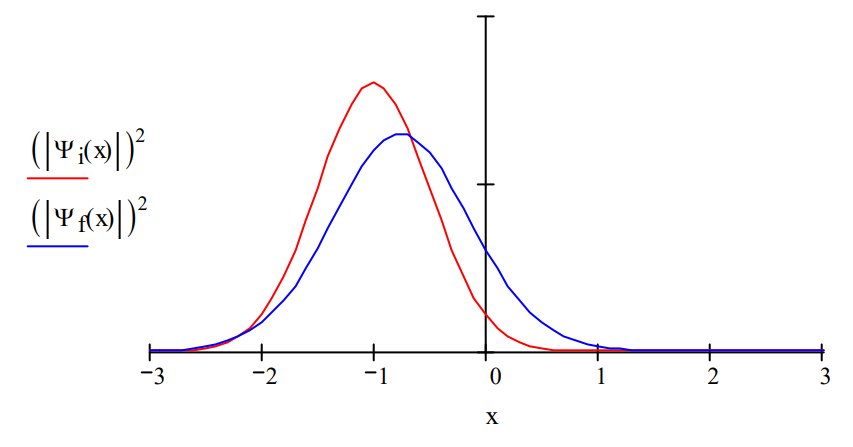
The initial wave function centered at x = ‐1 moves to the right under the influence of the harmonic oscillator potential as expected.

References:

1. John J. Tanner, “A Computer‐Based Approach to Teaching Quantum Dynamics,” J. Chem. Educ. 1990, 67, 917‐921.
2. John C. Hansen; Donald J. Kouri; David K. Hoffman, “A Spreadsheet Template for Quantum Mechanical Wavepacket Propagation,” J. Chem. Educ. 1997, 74, 335‐342.