
1.77: The Quantum Harmonic Oscillator
- Page ID
- 156478

The harmonic oscillator is frequently used by chemical educators as a rudimentary model for the vibrational degrees of freedom of diatomic molecules. Most often when this is done, the teacher is actually using a classical ball-and-spring model, or some hodge-podge hybrid of the classical and the quantum harmonic oscillator. Unfortunately these models are not accurate representations of the vibrational modes of molecules. To the extent that a simple harmonic potential can be used to represent molecular vibrational modes, it must be done in a pure quantum mechanical treatment based on solving the Schrödinger equation.
Schrödinger's equation in atomic units (h = 2\(\pi\)) for the harmonic oscillator has an exact analytical solution.
\[
\frac{-1}{2 \cdot \mu} \cdot \frac{\mathrm{d}^{2}}{\mathrm{dx}^{2}} \Psi(\mathrm{x})+\frac{1}{2} \cdot \mathrm{k} \cdot \mathrm{x}^{2} \cdot \Psi(\mathrm{x})=\mathrm{E} \cdot \Psi(\mathrm{x})
\nonumber \]
Potential energy:
\[
\mathrm{V}(\mathrm{x}, \mathrm{k}) :=\frac{1}{2} \cdot \mathrm{k} \cdot \mathrm{x}^{2}
\nonumber \]
Energy eigenstates:
\[
\mathrm{E}(\mathrm{v}, \mathrm{k}, \mu) :=\left(\mathrm{v}+\frac{1}{2}\right) \cdot \sqrt{\frac{\mathrm{k}}{\mu}}
\nonumber \]
Eigenfunctions:
\[
\Psi(x, v, k, \mu) :=\frac{(k \cdot \mu)^{\frac{1}{8}}}{\sqrt{2^{v} \cdot v ! \cdot \sqrt{\pi}}} \cdot \operatorname{Her}\left[v,(k \cdot \mu)^{\frac{1}{4}} \cdot x\right] \cdot \exp \left(\frac{\sqrt{k \cdot \mu \cdot x^{2}}}{2}\right)
\nonumber \]
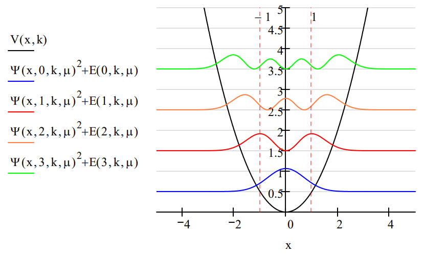
The probability distribution functions for k = \(\mu\) = 1 for the first four eigenstates are shown graphically below.
| Force constant: \(k : = 1\) | Effective mass: \(\mu : = 1\) |
The harmonic oscillator eigenfunctions form an orthonormal basis set.
Normalized:
\[
\int_{-\infty}^{\infty} \Psi(x, 0, k, \mu)^{2} d x=1
\nonumber \]
Orthogonal:
\[
\int_{-\infty}^{\infty} \Psi(x, 1, k, \mu) \cdot \Psi(x, 0, k, \mu) d x=0
\nonumber \]
Several non-classical attributes of the quantum oscillator are revealed in the graph above. Perhaps most obvious is that energy is quantized. Another is that the allowed oscillator states are stationary states. There is no vibratory motion associated with these states. In these allowed states, the oscillator is in a weighted superposition of all values of the x-coordinate, which in this case is the internuclear separation. The only time oscillatory motion occurs in the quantum oscillator is when it is perturbed by, for example, external electromagnetic radiation and making a transition from one allowed energy state to another. For a detailed discussion of these points see "Coherent Superpositions for the Harmonic Oscillator". For a discussion of "The Harmonic Oscillator and the Uncertainty Principle" visit this tutorial.
Another non-classical feature of the quantum oscillator is tunneling. The vertical dashed lines in the figure show the classical turning points for the ground state of the quantum oscillator. The classical turning point is that value of the x-coordinate at which the potential energy is equal to the total energy, and therefore classically the system must reverse its direction of motion.
Classical turning point for v=0, k=\(\mu\)=1:
\[
\frac{1}{2} \cdot \mathrm{k} \cdot \mathrm{x}^{2}=\left(\mathrm{v}+\frac{1}{2}\right) \cdot \sqrt{\frac{\mathrm{k}}{\mu}}\; \text{solve}, x\rightarrow \left[\begin{matrix} (2 \cdot v + 1)^{\frac{1}{2}} \\ -(2 \cdot v + 1)^{\frac{1}{2}}\end{matrix}\right] \text{substitute}, \mathrm{v}=0 \rightarrow\left(\begin{array}{c}{1} \\ {-1}\end{array}\right)
\nonumber \]
For v=0 the region beyond \(\pm\)1 is called the classically forbidden region because the oscillator does not have enough energy (E = 1/2) to be there because V > E. It implies a negative kinetic energy which does not make classical sense. Due to the symmetry of the potential well, the tunneling probability is calculated as follows.
\[
2 \cdot \int_{1}^{\infty} \Psi(x, 0, k, \mu)^{2} d x=0.157
\nonumber \]
It is easy to demonstrate that the tunneling probability decreases as the v quantum number increases. This might be considered a minor example of Bohr's correspondence principle: as the energy of a quantum system increases it appears to be more classical.
The fact that the wave functions of quantum states are superpositions is a fundamental idea in quantum theory. A quantum object (quon to use Nick Herbert's term) is not here or there, it is here and there. We can illuminate this idea by looking at a quantum oscillator's state operator, \(|\Psi><\Psi|\). This is also called the density operator or density matrix. It is a very powerful concept which is not generally presented in undergraduate courses in quantum physics or chemistry.
The state operator is now calculated and displayed for the v = 3 state. The state operator is a projection operator and its matrix elements, \(<\mathrm{x}_{1}|\Psi><\Psi| x_{2}>\), are calculated and displayed below. These matrix elements are the probability amplitude that an oscillator in the state \(| \Psi>\) is at both x1 and x2. This reveals the meaning of the quantum superposition as the quon being both here and there.
\[
\mathrm{v} :=3 \quad \operatorname{Min} :=5 \quad \mathrm{N} :=200 \quad \mathrm{j} :=0 \ldots \mathrm{N} \qquad \mathrm{k} :=0 \ldots \mathrm{N}
\nonumber \]
\[
x_{1_{j}} :=-\operatorname{Min}+\frac{2 \cdot \operatorname{Min} \cdot \mathrm{j}}{\mathrm{N}} \qquad \mathrm{x}_{2_{k}} :=-\operatorname{Min}+\frac{2 \cdot \mathrm{Min} \cdot \mathrm{k}}{\mathrm{N}}
\nonumber \]
\[
\Psi\left(x_{1}, x_{2}\right) :=\frac{1}{2^{v} \cdot v ! \cdot \sqrt{\pi}} \cdot \operatorname{Her}\left(v, x_{1}\right) \cdot \operatorname{Her}\left(v, x_{2}\right) \cdot \exp \left[\frac{-\left(x_{1}^{2}+x_{2}^{2}\right)}{2}\right] \\ \Psi \Psi_{j, k}=\Psi\left(x_{1}, x_{2}\right)
\nonumber \]
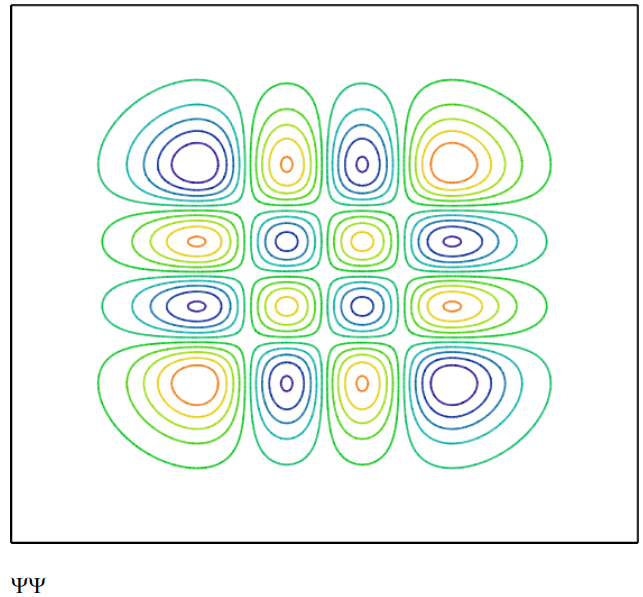
Viewing this as a graphical representation of the density matrix we clearly see the prominence of off-diagonal elements, elements with non-zero values for which x1 is not equal to x2. This is the signature of quantum mechanics. By comparison a classical system would have a diagonal density matrix - only the x1 = x2 elements would have non-zero values.
The following statements, modified slightly, are the best single-sentence descriptions of the meaning of the wave function I have read.
Quons are characterized by their entire distributions, called wave functions or orbitals, rather than by instantaneous positions and velocities: a quon may be considered always to be, with appropriate probability, at all points of its distribution, which does not vary with time. (F. E. Harris, Encyclopedia of Physics)
From the quantum mechanical perspective, to measure the position of a quon is not to find out where it is, but to cause it to be somewhere. (Louisa Gilder, The Age of Entanglement)