1.72: Superposition vs. Mixture

Last updated
Save as PDF

Page ID: 156462

\( \newcommand{\vecs}[1]{\overset { \scriptstyle \rightharpoonup} {\mathbf{#1}} } \) \( \newcommand{\vecd}[1]{\overset{-\!-\!\rightharpoonup}{\vphantom{a}\smash {#1}}} \)\(\newcommand{\id}{\mathrm{id}}\) \( \newcommand{\Span}{\mathrm{span}}\) \( \newcommand{\kernel}{\mathrm{null}\,}\) \( \newcommand{\range}{\mathrm{range}\,}\) \( \newcommand{\RealPart}{\mathrm{Re}}\) \( \newcommand{\ImaginaryPart}{\mathrm{Im}}\) \( \newcommand{\Argument}{\mathrm{Arg}}\) \( \newcommand{\norm}[1]{\| #1 \|}\) \( \newcommand{\inner}[2]{\langle #1, #2 \rangle}\) \( \newcommand{\Span}{\mathrm{span}}\) \(\newcommand{\id}{\mathrm{id}}\) \( \newcommand{\Span}{\mathrm{span}}\) \( \newcommand{\kernel}{\mathrm{null}\,}\) \( \newcommand{\range}{\mathrm{range}\,}\) \( \newcommand{\RealPart}{\mathrm{Re}}\) \( \newcommand{\ImaginaryPart}{\mathrm{Im}}\) \( \newcommand{\Argument}{\mathrm{Arg}}\) \( \newcommand{\norm}[1]{\| #1 \|}\) \( \newcommand{\inner}[2]{\langle #1, #2 \rangle}\) \( \newcommand{\Span}{\mathrm{span}}\)\(\newcommand{\AA}{\unicode[.8,0]{x212B}}\)

The Wigner function can be used to illustrate the difference between a superposition and a mixture. First consider the following linear superposition of Gaussian functions.

\[
\Psi(x) :=\exp \left[-(x-5)^{2}\right]+\exp \left[-(x+5)^{2}\right]
\nonumber \]

The Wigner distribution for this function is calculated and plotted below.

\[
\mathrm{W}(\mathrm{x}, \mathrm{p}) :=\int_{-\infty}^{\infty}\left[\exp \left[-\left(\mathrm{x}+\frac{\mathrm{s}}{2}-5\right)^{2}\right]+\exp \left[-\left(\mathrm{x}+\frac{\mathrm{s}}{2}+5\right)^{2}\right]\right] \cdot \exp (\mathrm{i} \cdot \mathrm{p} \cdot \mathrm{s}) \cdot\left[\exp \left[-\left(\mathrm{x}-\frac{\mathrm{s}}{2}-5\right)^{2}\right]+\exp \left[-\left(\mathrm{x}-\frac{\mathrm{s}}{2}+5\right)^{2}\right]\right] \mathrm{ds}
\nonumber \]

Integration yields:

\[
\mathrm{W}(\mathrm{x}, \mathrm{p}) :=\sqrt{2} \cdot \sqrt{\pi}\cdot\left(2 \cdot \exp \left(-2 \cdot \mathrm{x}^{2}-\frac{1}{2} \cdot \mathrm{p}^{2}\right) \cdot \cos (10 \cdot \mathrm{p})+\exp \left(-2 \cdot x^{2}+20 \cdot x-50-\frac{1}{2} \cdot p^{2}\right)+\exp \left(-2 \cdot x^{2}-20 \cdot x-50-\frac{1}{2} \cdot p^{2}\right)\right)
\nonumber \]

\[
\mathrm{N} :=50 \qquad \mathrm{i} :=0 \ldots \mathrm{N} \qquad \mathrm{x}_{\mathrm{i}} :=-7+\frac{14 \cdot \mathrm{i}}{\mathrm{N}} \\ \mathrm{j} :=0 \ldots \mathrm{N} \qquad \mathrm{p}_{\mathrm{j}} :=-6+\frac{12 \cdot \mathrm{j}}{\mathrm{N}} \qquad \text{Wigner}_{\mathrm{i}, \mathrm{j}} :=\mathrm{W}\left(\mathrm{x}_{\mathrm{i}}, \mathrm{p}_{\mathrm{j}}\right)
\nonumber \]

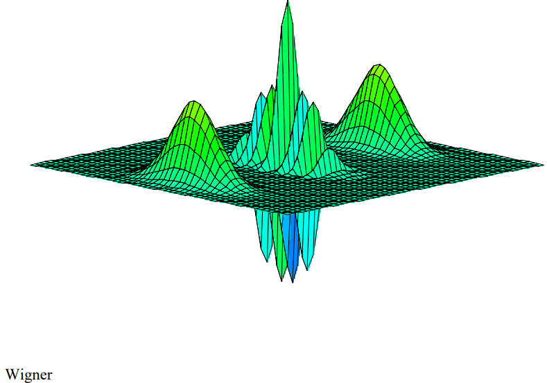
The signature of a superposition is the occurrence of interference fringes as seen in the center of the figure above.

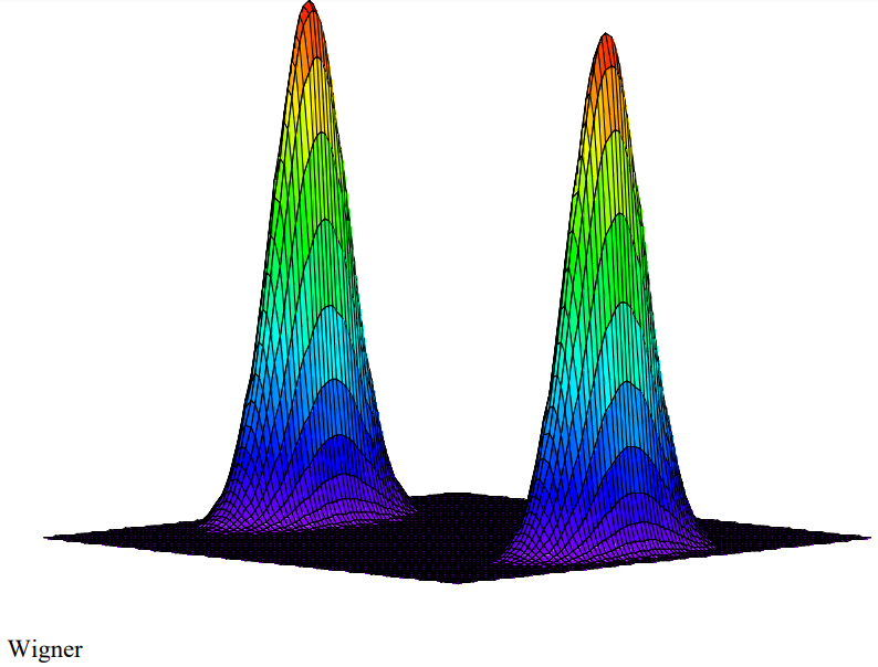
The Wigner function for a classical mixture is the sum of Wigner functions for each member of the mixture. The interference region is clearly absent in the figure shown below.

\[
\mathrm{W}(\mathrm{x}, \mathrm{p}) :=\int_{-\infty}^{\infty} \exp \left[-\left(\mathrm{x}+\frac{\mathrm{s}}{2}-5\right)^{2}\right] \cdot \exp (\mathrm{i} \cdot \mathrm{p} \cdot \mathrm{s}) \cdot \exp \left[-\left(\mathrm{x}-\frac{\mathrm{s}}{2}-5\right)^{2}\right] \mathrm{ds}+\int_{-\infty}^{\infty} \exp \left[-\left(x+\frac{s}{2}+5\right)^{2}\right] \cdot \exp (i \cdot p \cdot s) \cdot \exp \left[-\left(x-\frac{s}{2}+5\right)^{2}\right] d s
\nonumber \]

Integration yields:

\[
\mathrm{W}(\mathrm{x}, \mathrm{p}) :=\exp \left(-2 \cdot \mathrm{x}^{2}+20 \cdot \mathrm{x}-50-\frac{1}{2} \cdot \mathrm{p}^{2}\right) \cdot \sqrt{2} \cdot \sqrt{\pi}+\exp \left(-2 \cdot \mathrm{x}^{2}-20 \cdot \mathrm{x}-50-\frac{1}{2} \cdot \mathrm{p}^{2}\right) \cdot \sqrt{2} \cdot \sqrt{\pi}
\nonumber \]

\[
\mathrm{N} :=100 \qquad \mathrm{i} :=0 \ldots \mathrm{N} \qquad \mathrm{x}_{\mathrm{i}} :=-7+\frac{14 \cdot \mathrm{i}}{\mathrm{N}} \\ \mathrm{j} :=0 \ldots \mathrm{N} \qquad \mathrm{p}_{\mathrm{j}} :=-6+\frac{12 \cdot \mathrm{j}}{\mathrm{N}} \qquad \text{Wigner}_{i, j} :=\mathrm{W}\left(\mathrm{x}_{i}, \mathrm{p}_{j}\right)
\nonumber \]

Reference: Decoherence and the Transition form Quantum to Classical, Wojciech Jurek, Physics Today, October 1991, pages 36-44.