1.70: Wigner Distribution for the Particle in a Box

Last updated
Save as PDF

Page ID: 156420

\( \newcommand{\vecs}[1]{\overset { \scriptstyle \rightharpoonup} {\mathbf{#1}} } \) \( \newcommand{\vecd}[1]{\overset{-\!-\!\rightharpoonup}{\vphantom{a}\smash {#1}}} \)\(\newcommand{\id}{\mathrm{id}}\) \( \newcommand{\Span}{\mathrm{span}}\) \( \newcommand{\kernel}{\mathrm{null}\,}\) \( \newcommand{\range}{\mathrm{range}\,}\) \( \newcommand{\RealPart}{\mathrm{Re}}\) \( \newcommand{\ImaginaryPart}{\mathrm{Im}}\) \( \newcommand{\Argument}{\mathrm{Arg}}\) \( \newcommand{\norm}[1]{\| #1 \|}\) \( \newcommand{\inner}[2]{\langle #1, #2 \rangle}\) \( \newcommand{\Span}{\mathrm{span}}\) \(\newcommand{\id}{\mathrm{id}}\) \( \newcommand{\Span}{\mathrm{span}}\) \( \newcommand{\kernel}{\mathrm{null}\,}\) \( \newcommand{\range}{\mathrm{range}\,}\) \( \newcommand{\RealPart}{\mathrm{Re}}\) \( \newcommand{\ImaginaryPart}{\mathrm{Im}}\) \( \newcommand{\Argument}{\mathrm{Arg}}\) \( \newcommand{\norm}[1]{\| #1 \|}\) \( \newcommand{\inner}[2]{\langle #1, #2 \rangle}\) \( \newcommand{\Span}{\mathrm{span}}\)\(\newcommand{\AA}{\unicode[.8,0]{x212B}}\)

The Wigner function is a quantum mechanical phase-space quasi-probability function. It is called a quasi-probability function because it can take on negative values, which have no classical meaning in terms of probability.

The PIB eigenstates for a box of unit dimension are given by:

\[
\Psi(x, n) :=\sqrt{2} \cdot \sin (n \cdot \pi \cdot x)
\nonumber \]

For these eigenstates the Wigner distribution function is:

\[
\mathrm{W}(\mathrm{x}, \mathrm{p}, \mathrm{n}) :=\frac{1}{\pi} \cdot \int_{-\mathrm{x}}^{\mathrm{x}} \sqrt{2} \cdot \sin [\mathrm{n} \cdot \pi \cdot(\mathrm{x}+\mathrm{s})] \cdot \exp (2 \cdot \mathrm{i} \cdot \mathrm{s} \cdot \mathrm{p}) \cdot \sqrt{2} \cdot \sin [\mathrm{n} \cdot \pi \cdot(\mathrm{x}-\mathrm{s})] \mathrm{ds}
\nonumber \]

Integration with respect to s yields the following function:

\[
\mathrm{W}(\mathrm{x}, \mathrm{p}, \mathrm{n}) :=\frac{2}{\pi} \cdot\left[\frac{\sin [2 \cdot(\mathrm{p}-\mathrm{n} \cdot \pi) \cdot \mathrm{x}]}{4 \cdot(\mathrm{p}-\mathrm{n} \cdot \pi)}+\frac{\sin [2 \cdot(\mathrm{p}+\mathrm{n} \cdot \pi) \cdot \mathrm{x}]}{4 \cdot(\mathrm{p}+\mathrm{n} \cdot \pi)}-\cos (2 \cdot \mathrm{n} \cdot \pi \cdot \mathrm{x}) \cdot \frac{\sin (2 \cdot p \cdot \mathrm{x})}{2 \cdot p}\right]
\nonumber \]

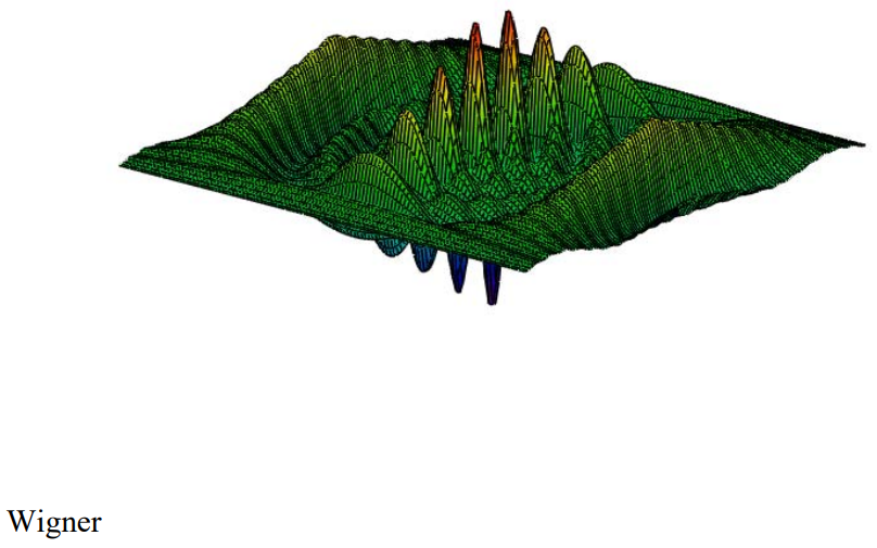
The Wigner distribution for the nth eigenstate is calculated below:

\[
\mathrm{n} :=10 \qquad \mathrm{N} :=115 \qquad \mathrm{i} :=0 . . \mathrm{N} \\ \mathrm{x}_{\mathrm{i}} :=\frac{\mathrm{i}}{\mathrm{N}} \qquad \mathrm{j} :=0 . . \mathrm{N} \qquad \mathrm{p}_{\mathrm{j}} :=-40+\frac{80 \cdot \mathrm{j}}{\mathrm{N}}
\nonumber \]

\[
\text{Wigner}_{i, j} :=\operatorname{if}\left[x_{i} \leq 0.5, W\left(x_{i}, p_{j}, n\right), W\left[\left(1-x_{i}\right), p_{j}, n\right]\right]
\nonumber \]

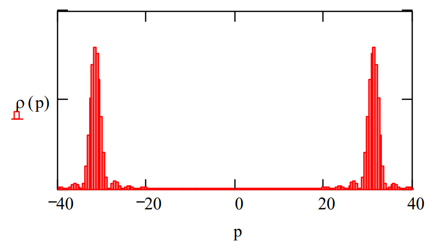
Integration of the Wigner function over the spatial coordinate yields the momentum distribution function as is shown below.

\[
\rho(\mathrm{p}) :=\int_{0}^{1} \mathrm{W}(\mathrm{x}, \mathrm{p}, \mathrm{n}) \mathrm{dx} \qquad \mathrm{p} :=-40,-39.5 \ldots40
\nonumber \]

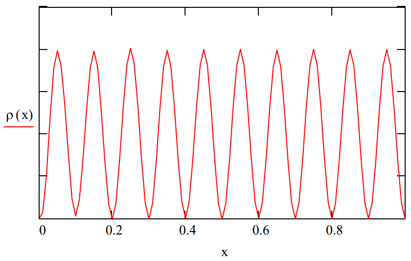
Integration of the Wigner function over the momentum coordinate yields the spatial distribution function as is shown below.

\[
\rho(\mathrm{x}) :=\int_{-51}^{50} \mathrm{W}(\mathrm{x}, \mathrm{p}, \mathrm{n}) \mathrm{dp} \qquad \mathrm{x} :=0,01 \ldots 1
\nonumber \]

The Wigner distribution can be used to calculate the expectation values for position, momentum and kinetic energy.

\[
\mathrm{x}_{\mathrm{bar}}=\int_{-\infty}^{\infty} \int_{0}^{1} \mathrm{W}(\mathrm{x}, \mathrm{p}, 1) \cdot \mathrm{x} \text { dx dp simplify } \rightarrow \mathrm{x}_{\mathrm{bar}}=\frac{1}{2}
\nonumber \]

\[
\mathrm{p}_{\mathrm{bar}}=\int_{-\infty}^{\infty} \int_{0}^{1} \mathrm{W}(\mathrm{x}, \mathrm{p}, 1) \cdot \mathrm{p} \mathrm{dx} \text { dp simplify } \rightarrow \mathrm{p}_{\mathrm{bar}}=0
\nonumber \]

\[
\mathrm{T}_{\mathrm{bar}}=\int_{-\infty}^{\infty} \int_{0}^{1} \mathrm{W}(\mathrm{x}, \mathrm{p}, 1) \cdot \frac{\mathrm{p}^{2}}{2} \mathrm{d} \mathrm{x} \text { dp simplify } \rightarrow \mathrm{T}_{\mathrm{bar}}=\frac{1}{2} \cdot \pi^{2}
\nonumber \]

References:

"Wigner quasi-probability distribution for the infinite square well: Energy eigenstates and time-dependent wave packets," by Belloni, Docheski and Robinett; American Journal of Physics 72(9), 1183-1192 (2004).

"Wigner functions and Weyl transforms for pedestrians," by William Case, American Journal of Physics 76(10), 937-946 (2008).