1.45: Terse Analysis of Triple-slit Diffraction with a Quantum Eraser
- Page ID
- 149263

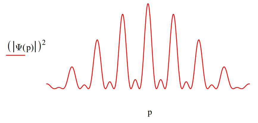
Slit positions, slit width and the wavefunction at the slit screen which is a superposition of the photon being simultaneously present at all three slits.
\[
\mathrm{x}_{1} :=-\frac{1}{2} \quad \mathrm{x}_{2} :=0 \quad \mathrm{x}_{3} :=\frac{1}{2} \quad \delta :=0.1
\nonumber \]
\[
| \Psi \rangle=\frac{1}{\sqrt{3}}\left[ | x_{1}\right\rangle+| x_{2} \rangle+| x_{3} \rangle ]
\nonumber \]
Calculate the diffraction pattern by a Fourier transform of the spatial wavefunction into momentum space.
\[
\langle p | \Psi\rangle=\frac{1}{\sqrt{3}}\left[\left\langle p | x_{1}\right\rangle+\left\langle p | x_{2}\right\rangle+\left\langle p | x_{3}\right\rangle\right]
\nonumber \]
\[
\Psi(\mathrm{p}) := \int_{\mathrm{x}_{1}-\frac{\delta}{2}}^{\mathrm{x}_{1}+\frac{\delta}{2}} \frac{1}{\sqrt{2 \cdot \pi}} \cdot \exp (-\mathrm{i} \cdot \mathrm{p} \cdot \mathrm{x}) \cdot \frac{1}{\sqrt{\delta}} \mathrm{d} \mathrm{x} +\int_{\mathrm{x}_{2}-\frac{\delta}{2}}^{\mathrm{x}_{2}+\frac{\delta}{2}} \frac{1}{\sqrt{2 \cdot \pi}} \cdot \exp (-\mathrm{i} \cdot \mathrm{p} \cdot \mathrm{x}) \cdot \frac{1}{\sqrt{\delta}} \mathrm{dx} +\int_{\mathrm{x}_{3}-\frac{\delta}{2}}^{\mathrm{x}_{3}+\frac{\delta}{2}} \frac{1}{\sqrt{2 \cdot \pi}} \cdot \exp (-\mathrm{i} \cdot \mathrm{p} \cdot \mathrm{x}) \cdot \frac{1}{\sqrt{\delta}} \mathrm{dx}
\nonumber \]
Display the momentum distribution function which is the diffraction pattern.
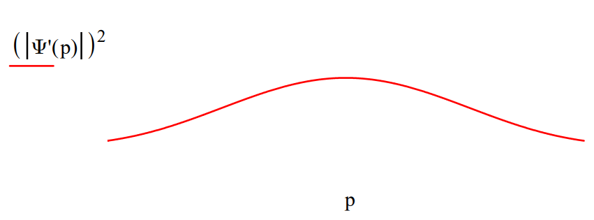
Tag the slits with orthogonal states.
\[
\left\langle p | \Psi^{\prime}\right\rangle=\frac{1}{\sqrt{3}}\left[\left\langle p | x_{1}\right\rangle | \uparrow\right\rangle+\left\langle p | x_{2}\right\rangle | \rightarrow \rangle+\left\langle p | x_{3}\right\rangle | \downarrow \rangle ]
\nonumber \]
Recalculate the momentum distribution.
\[
\Psi^{\prime}(\mathrm{p}) :=\int_{\mathrm{x}_{1} \frac{\delta}{2}}^{\mathrm{x}_{1}+\frac{\delta}{2}} \frac{1}{\sqrt{2 \cdot \pi}} \cdot \exp (-\mathrm{i} \cdot \mathrm{p} \cdot \mathrm{x}) \cdot \frac{1}{\sqrt{\delta}} \mathrm{d} x \cdot \left( \begin{array}{l}{1} \\ {0} \\ {0}\end{array}\right)+ \\ \int_{\mathrm{x}_{2}-\frac{\delta}{2}}^{\mathrm{x}_{2}+\frac{\delta}{2}} \frac{1}{\sqrt{2 \cdot \pi}} \cdot \exp (-\mathrm{i} \cdot \mathrm{p} \cdot \mathrm{x}) \cdot \frac{1}{\sqrt{\delta}} \mathrm{d} \mathrm{x} \cdot \left( \begin{array}{l}{0} \\ {1} \\ {0}\end{array}\right)+\int_{\mathrm{x}_{3}-\frac{\delta}{2}}^{\mathrm{x}_{3}+\frac{\delta}{2}} \frac{1}{\sqrt{2 \cdot \pi}} \cdot \exp (-\mathrm{i} \cdot \mathrm{p} \cdot \mathrm{x}) \cdot \frac{1}{\sqrt{\delta}} \mathrm{d} \mathrm{x} \cdot \left( \begin{array}{l}{0} \\ {0} \\ {1}\end{array}\right)
\nonumber \]
Display the momentum distribution at the detection screen showing that the diffraction pattern has disappeared. The orthogonallity of the tags destroys the cross-terms in the momentum distribution, \left|\Psi^{\prime}(\mathrm{p})\right|^{2}, which give rise to the interference effects shown in the original diffraction pattern.
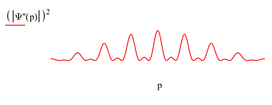
Insert an "eraser" after the slit screen and before the detection screen.
\[
\Psi^{\prime \prime}(\mathrm{p}) :=\frac{1}{\sqrt{3}} \cdot \left( \begin{array}{l}{1} \\ {1} \\ {1}\end{array}\right)^{\mathrm{T}} . \Psi^{\prime}(\mathrm{p})
\nonumber \]
The diffraction pattern is restored but attenuated because the so-called "eraser" filters out the orthogonal tags restoring the interference terms.