1.11: Quantum Computation- A Short Course
- Page ID
- 140080

The four remaining tutorials deal with this clash between quantum mechanics and local realism, and the simulation of physical phenomena. The first two examine entangled spin systems and the third entangled photon systems. The fourth provides a terse mathematical summary for both spin and photon systems. They all clearly show the disagreement between the predictions of quantum theory and those of local hidden-variable models.
Another Look at Mermin's EPR Gedanken Experiment
Quantum theory is both stupendously successful as an account of the small-scale structure of the world and it is also the subject of an unresolved debate and dispute about its interpretation. J. C. Polkinghorne, The Quantum World, p. 1.
In Bohm's EPR thought experiment (Quantum Theory, 1951, pp. 611-623), both local realism and quantum mechanics were shown to be consistent with the experimental data. However, the local realistic explanation used composite spin states that were invalid according to quantum theory. The local realists countered that this was an indication that quantum mechanics was incomplete because it couldn't assign well-defined values to all observable properties prior to or independent of observation. In the 1980s N. David Mermin presented a related thought experiment [American Journal of Physics (October 1981, pp 941-943) and Physics Today (April 1985, pp 38-47)] in which the predictions of local realism and quantum mechanics disagree. As such Mermin's thought experiment represents a specific illustration of Bell's theorem.
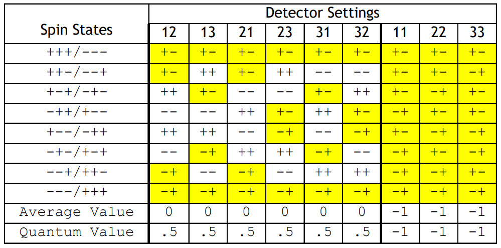
A spin-1/2 pair is prepared in a singlet state and the individual particles travel in opposite directions to detectors which are set up to measure spin in three directions in x-z plane: along the z-axis, and angles of 120 and 240 degrees with respect to the z-axis. The detector settings are labeled 1, 2 and 3, respectively.
The switches on the detectors are set randomly so that all nine possible settings of the two detectors occur with equal frequency.
Local realism holds that objects have properties independent of measurement and that measurements at one location on a particle cannot influence measurements of another particle at a distant location even if the particles were created in the same event. Local realism maintains that the spin-1/2 particles carry instruction sets (hidden variables) which dictate the results of subsequent measurements. Prior to measurement the particles are in an unknown but well-defined state.
The following table presents the experimental results expected on the basis of local realism. Singlet spin states have opposite spin values for each of the three measurement directions. If A's spin state is (+-+), then B's spin state is (-+-). A '+' indicates spin-up and a measurement eigenvalue of +1. A '-' indicates spin-down and a measurement eigenvalue of -1. If A's detector is set to spin direction "1" and B's detector is set to spin direction "3" the measured result will be recorded as +-,with an eigenvalue of -1.
There are eight spin states and nine possible detector settings, giving 72 possible measurement outcomes all of which are equally probable. The next to bottom line of the table shows the average (expectation) value for the nine possible detector settings given the local realist spin states. When the detector settings are the same there is perfect anti-correlation between the detectors at A and B. When the detectors are set at different spin directions there is no correlation.
As will now be shown quantum mechanics (bottom line of the table) disagrees with this local realistic analysis. The singlet state produced by the source is the following entangled superposition, where the arrows indicate the spin orientation for any direction in the x-z plane. As noted above the directions used are 0, 120 and 240 degrees, relative to the z-axis.
\[
| \Psi \rangle=\frac{1}{\sqrt{2}}[ |\uparrow\rangle_{1} | \downarrow \rangle_{2}-| \downarrow \rangle_{1} | \uparrow \rangle_{2} ]=\frac{1}{\sqrt{2}}\left[\left( \begin{array}{c}{\cos \left(\frac{\varphi}{2}\right)} \\ {\sin \left(\frac{\varphi}{2}\right)}\end{array}\right) \otimes \left( \begin{array}{c}{-\sin \left(\frac{\varphi}{2}\right)} \\ {\cos \left(\frac{\varphi}{2}\right)}\end{array}\right)-\left( \begin{array}{c}{-\sin \left(\frac{\varphi}{2}\right)} \\ {\cos \left(\frac{\varphi}{2}\right)}\end{array}\right) \otimes \left( \begin{array}{c}{\cos \left(\frac{\varphi}{2}\right)} \\ {\sin \left(\frac{\varphi}{2}\right)}\end{array}\right)\right]=\frac{1}{\sqrt{2}} \left( \begin{array}{c}{0} \\ {1} \\ {-1} \\ {0}\end{array}\right) \quad \Psi :=\frac{1}{\sqrt{2}} \cdot \left( \begin{array}{c}{0} \\ {1} \\ {-1} \\ {0}\end{array}\right)
\nonumber \]
The single particle spin operator in the x-z plane is constructed from the Pauli spin operators in the xand z-directions. \(\phi\) is the angle of orientation of the measurement magnet with the z-axis. Note that the Pauli operators measure spin in units of \frac{h}{4 \pi}\). This provides for some mathematical clarity in the forthcoming analysis.
\[
\sigma_{\mathrm{Z}} :=\left( \begin{array}{cc}{1} & {0} \\ {0} & {-1}\end{array}\right) \qquad \sigma_{\mathrm{x}} :=\left( \begin{array}{ll}{0} & {1} \\ {1} & {0}\end{array}\right) \\ \mathrm{S}(\varphi) :=\cos (\varphi) \cdot \sigma_{\mathrm{Z}}+\sin (\varphi) \cdot \sigma_{\mathrm{x}} \rightarrow \left( \begin{array}{cc}{\cos (\varphi)} & {\sin (\varphi)} \\ {\sin (\varphi)} & {-\cos (\varphi)}\end{array}\right)
\nonumber \]
The joint spin operator for the two-spin system in tensor format is,
\[
\left( \begin{array}{cc}{\cos \varphi_{A}} & {\sin \varphi_{A}} \\ {\sin \varphi_{A}} & {-\cos \varphi_{A}}\end{array}\right) \otimes \left( \begin{array}{cc}{\cos \varphi_{B}} & {\sin \varphi_{B}} \\ {\sin \varphi_{B}} & {-\cos \varphi_{B}}\end{array}\right)= \begin{pmatrix} \cos \varphi_{A} \left( \begin{array}{cc}{\cos \varphi_{B}} & {\sin \varphi_{B}} \\ {\sin \varphi_{B}} & {-\cos \varphi_{B}}\end{array}\right) & \sin \varphi_{A} \left( \begin{array}{cc}{\cos \varphi_{B}} & {\sin \varphi_{B}} \\ {\sin \varphi_{B}} & {-\cos \varphi_{B}}\end{array}\right) \\ \sin \varphi_{A} \left( \begin{array}{cc}{\cos \varphi_{B}} & {\sin \varphi_{B}} \\ {\sin \varphi_{B}} & {-\cos \varphi_{B}}\end{array}\right) & -\cos \varphi_{A} \left( \begin{array}{cc}{\cos \varphi_{B}} & {\sin \varphi_{B}} \\ {\sin \varphi_{B}} & {-\cos \varphi_{B}}\end{array}\right) \end{pmatrix}
\nonumber \]
In Mathcad syntax this operator is:
\[
\mathrm{kronecker}\left(\mathrm{S}\left(\varphi_{\mathrm{A}}\right), \mathrm{S}\left(\varphi_{\mathrm{B}}\right)\right)
\nonumber \]
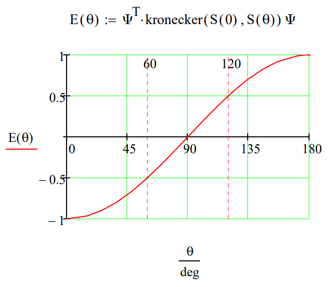
When the detector settings are the same quantum theory predicts an expectation value of -1, in agreement with the analysis based on local realism.
\[
\Psi^{\mathrm{T}} \cdot \text { kronecker }(\mathrm{S}(0 \cdot \mathrm{deg}), \mathrm{S}(0 \cdot \mathrm{deg})) \Psi=-1 \quad \Psi^{\mathrm{T}} \cdot \text { kronecker }(\mathrm{S}(120 \cdot \mathrm{deg}), \mathrm{S}(120 \cdot \mathrm{deg})) \Psi=-1 \quad \Psi^{T} \cdot \text { kronecker }(\mathrm{S}(240 \cdot \text { deg }), \mathrm{S}(240 \cdot \mathrm{deg})) \Psi=-1
\nonumber \]
However, when the detector settings are different quantum theory predicts an expectation value of 0.5, in disagreement with the local realistic value of 0.
\[
\Psi^{\mathrm{T}} \cdot \text { kronecker }(\mathrm{S}(0 \cdot \mathrm{deg}), \mathrm{S}(120 \cdot \mathrm{deg})) \Psi=0.5 \quad \Psi^{T} \cdot \text { kronecker }(\mathrm{S}(0 \cdot \operatorname{deg}), \mathrm{S}(240 \cdot \mathrm{deg})) \Psi=0.5 \quad \Psi^{\mathrm{T}} \cdot \text { kronecker }(\mathrm{S}(120 \cdot \mathrm{deg}), \mathrm{S}(240 \cdot \mathrm{deg})) \Psi=0.5
\nonumber \]
Considering all detector settings local realism predicts an expectation value of -1/3 [2/3(0) + 1/3(-1)], while quantum theory predicts an expectation value of 0 [2/3(1/2) + 1/3(-1)]. (See the two bottom rows in the table above.)
Furthermore, the following calculations demonstrate that the various spin operators do not commute and therefore represent incompatible observables. In other words, they are observables that cannot simultaneously be in well-defined states. Thus, quantum theory also rejects the realist's spin states used in the table.
\[
\mathrm{S}(0 \cdot \operatorname{deg}) \cdot \mathrm{S}(120 \cdot \mathrm{deg})-\mathrm{S}(120 \cdot \mathrm{deg}) \cdot \mathrm{S}(0 \cdot \mathrm{deg})=\left( \begin{array}{cc}{0} & {1.732} \\ {-1.732} & {0}\end{array}\right)
\nonumber \]
\[
\mathrm{S}(0 \cdot \mathrm{deg}) \cdot \mathrm{S}(240 \cdot \mathrm{deg})-\mathrm{S}(240 \cdot \mathrm{deg}) \cdot \mathrm{S}(0 \cdot \mathrm{deg})=\left( \begin{array}{cc}{0} & {-1.732} \\ {1.732} & {0}\end{array}\right)
\nonumber \]
\[
\mathrm{S}(120 \cdot \mathrm{deg}) \cdot \mathrm{S}(240 \cdot \mathrm{deg})-\mathrm{S}(240 \cdot \mathrm{deg}) \cdot \mathrm{S}(120 \cdot \mathrm{deg})=\left( \begin{array}{cc}{0} & {1.732} \\ {-1.732} & {0}\end{array}\right)
\nonumber \]
The local realist is undeterred by this argument and the disagreement with the quantum mechanical predictions, asserting that the fact that quantum theory cannot assign well-defined states to all elements of reality independent of observation is an indication that it provides an incomplete description of reality.
However, results available for experiments of this type with photons support the quantum mechanical predictions and contradict the local realists analysis shown in the table above. Thus, there appears to be a non-local interaction between the two spins at their measurement sites. Nick Herbert provides a memorable and succinct description of such non-local influences on page 214 of Quantum Reality.
A non-local interaction links up one location with another without crossing space, without decay, and without delay. A non-local interaction is, in short, unmediated, unmitigated, and immediate.
Jim Baggott puts it this way (The Meaning of Quantum Theory, page 135):
The predictions of quantum theory (in this experiment) are based on the properties of a two-particle state vector which ... is 'delocalized' over the whole experimental arrangement. The two particles are, in effect, always in 'contact' prior to measurement and can therefore exhibit a degree of correlation that is impossible for two Einstein separable particles.
"...if [a hidden-variable theory] is local it will not agree with quantum mechanics, and if it agrees with quantum mechanics it will not be local. This is what the theorem says." -John S. Bell
Further Information
The eigenvectors of the single particle spin operator, S(\(phi\)), in the x-z plane are given below along with their eigenvalues.
\[
\varphi_{u}(\varphi) :=\left( \begin{array}{c}{\cos \left(\frac{\varphi}{2}\right)} \\ {\sin \left(\frac{\varphi}{2}\right)}\end{array}\right) \qquad \varphi_{\mathrm{d}}(\varphi) :=\left( \begin{array}{c}{-\sin \left(\frac{\varphi}{2}\right)} \\ {\cos \left(\frac{\varphi}{2}\right)}\end{array}\right)
\nonumber \]
\[
\varphi_{\mathrm{u}}(\varphi)^{\mathrm{T}} \cdot \varphi_{\mathrm{u}}(\varphi) \text { simplify } \rightarrow 1 \quad \varphi_{\mathrm{d}}(\varphi)^{\mathrm{T}} \cdot \varphi_{\mathrm{d}}(\varphi) \text { simplify } \rightarrow 1 \quad \varphi_{\mathrm{d}}(\varphi)^{\mathrm{T}} \cdot \varphi_{\mathrm{u}}(\varphi) \text { simplify } \rightarrow 0
\nonumber \]
| Eigenvalue +1 | Eigenvalue -1 |
|---|---|
| $$\mathrm{S}(\varphi) \cdot \varphi_{\mathrm{u}}(\varphi) \text { simplify } \rightarrow \left( \begin{array}{c}{\cos \left(\frac{\varphi}{2}\right)} \\ {\sin \left(\frac{\varphi}{2}\right)}\end{array}\right)$$ | $$\mathrm{S}(\varphi) \cdot \varphi_{\mathrm{d}}(\varphi) \text { simplify } \rightarrow \left( \begin{array}{c}{\sin \left(\frac{\varphi}{2}\right)} \\ {-\cos \left(\frac{1}{2} \cdot \varphi\right)}\end{array}\right) $$ |
A summary of the quantum mechanical calculations:
\[\begin{pmatrix} \Psi^{T} \cdot \text { kronecker }(\mathrm{S}(0 \cdot \operatorname{deg}), \mathrm{S}(120 \cdot \mathrm{deg})) \Psi \\ \Psi^{T} \cdot \text { kronecker }(\mathrm{S}(0 \cdot \operatorname{deg}), \mathrm{S}(240 \cdot \mathrm{deg})) \Psi \\ \Psi^{T} \cdot \text { kronecker }(\mathrm{S}(120 \cdot \operatorname{deg}), \mathrm{S}(0 \cdot \mathrm{deg})) \Psi \\ \Psi^{T} \cdot \text { kronecker }(\mathrm{S}(120 \cdot \operatorname{deg}), \mathrm{S}(240 \cdot \mathrm{deg})) \Psi \\ \Psi^{T} \cdot \text { kronecker }(\mathrm{S}(240 \cdot \operatorname{deg}), \mathrm{S}(0 \cdot \mathrm{deg})) \Psi \\ \Psi^{T} \cdot \text { kronecker }(\mathrm{S}(240 \cdot \operatorname{deg}), \mathrm{S}(120 \cdot \mathrm{deg})) \Psi \\ \Psi^{T} \cdot \text { kronecker }(\mathrm{S}(0 \cdot \operatorname{deg}), \mathrm{S}(0 \cdot \mathrm{deg})) \Psi \\ \Psi^{T} \cdot \text { kronecker }(\mathrm{S}(120 \cdot \operatorname{deg}), \mathrm{S}(120 \cdot \mathrm{deg})) \Psi \\ \Psi^{T} \cdot \text { kronecker }(\mathrm{S}(240 \cdot \operatorname{deg}), \mathrm{S}(240 \cdot \mathrm{deg})) \Psi \end{pmatrix}^{T}=\left( \begin{array}{cccccccc}{0.5} & {0.5} & {0.5} & {0.5} & {0.5} & {0.5} & {-1} & {-1} & {-1}\end{array}\right) \nonumber \]
Calculation of the overall spin expectation value:
\[
\sum_{i=0}^{2} \sum_{j=0}^{2} \left[\Psi^{\mathrm{T}} \cdot \text { kronecker }[\mathrm{S}[\mathrm{i} \cdot(120 \cdot \mathrm{deg})], \mathrm{S}[j \cdot(120 \cdot \mathrm{deg})]] \Psi\right]=0
\nonumber \]
The expectation value as a function of the relative orientation of the detectors reveals the level of correlation between the two spin measurements. For \(\theta\) = 0° there is perfect anti-correlation; for \(\theta\) = 180° perfect correlation; for \(\theta\) = 90° no correlation; for \(\theta\) = 60° intermediate anti-correlation (-0.5) and for \(\theta\) = 120° intermediate correlation (0.5).
A Quantum Simulation
This thought experiment is simulated using the following quantum circuit. As shown below the results are in agreement with the previous theoretical quantum calculations. The initial Hadamard and CNOT gates create the singlet state from the |11> input. Rz(\(\theta\)) rotates spin B. The final Hadamard gates prepare the system for measurement. See arXiv:1712.05642v2 for further detail.
\[\begin{matrix} \text{Spin A} & | 1 \rangle & \rhd & H & \cdot & \cdots & H & \rhd & \text{Measure 0 or 1: Eigenvalue 1 or -1} \\ \; & \; & \; & \; & | & \; & \; & \; & \; \\ \text{Spin B} & | 1 \rangle & \rhd & \cdots & \oplus & R_{Z} (\theta) & H & \rhd & \text{Measure 0 or 1: Eigenvalue 1 or -1} \end{matrix} \nonumber \]
The quantum gates required to execute this circuit:
| Identity | Hadamard gate | Rz rotation | Controlled NOT |
|---|---|---|---|
| $$\mathrm{I} :=\left( \begin{array}{ll}{1} & {0} \\ {0} & {1}\end{array}\right)$$ | $$\mathrm{H} :=\frac{1}{\sqrt{2}} \cdot \left( \begin{array}{cc}{1} & {1} \\ {1} & {-1}\end{array}\right) $$ | $$ \mathrm{R}_{\mathrm{Z}}(\theta) :=\left( \begin{array}{cc}{1} & {0} \\ {0} & {\mathrm{e}^{\mathrm{i} \cdot \theta}}\end{array}\right)$$ | $$\mathrm{CNOT} :=\left( \begin{array}{cccc}{1} & {0} & {0} & {0} \\ {0} & {1} & {0} & {0} \\ {0} & {0} & {0} & {1} \\ {0} & {0} & {1} & {0}\end{array}\right)$$ |
The operator representing the circuit is constructed from the matrix operators provided above.
\[
\mathrm{Op}(\theta) :=\text { kronecker }(\mathrm{H}, \mathrm{H}) \cdot \text { kronecker }\left(\mathrm{I}, \mathrm{R}_{\mathrm{Z}}(\theta)\right) \text { CNOT kronecker }(\mathrm{H}, \mathrm{I})
\nonumber \]
There are four equally likely measurement outcomes with the eigenvalues and overall expectation values shown below for relative measurement angles 0 and 120 deg (\(\frac{2 \pi}{3}\)).
| |00> eigenvalue +1 |
$$ \left[\left|\left( \begin{array}{c}{1} \\ {0} \\ {0} \\ {0}\end{array}\right)^{\mathrm{T}} \cdot \mathrm{Op}(0 \cdot \mathrm{deg}) \cdot \left( \begin{array}{l}{0} \\ {0} \\ {0} \\ {1}\end{array}\right)\right|\right]^{2}=0 $$ |
|01> eigenvalue -1 |
$$ \left[\left|\left( \begin{array}{l}{0} \\ {1} \\ {0} \\ {0}\end{array}\right)^{\mathrm{T}} \cdot \operatorname{Op}(0 \cdot \operatorname{deg}) \cdot \left( \begin{array}{l}{0} \\ {0} \\ {0} \\ {1}\end{array}\right)\right|\right]^{2}=0.5 $$ |
| |10> eigenvalue -1 |
$$ \left[\left|\left( \begin{array}{c}{0} \\ {0} \\ {1} \\ {0}\end{array}\right)^{\mathrm{T}} \cdot \mathrm{Op}(0 \cdot \mathrm{deg}) \cdot \left( \begin{array}{l}{0} \\ {0} \\ {0} \\ {1}\end{array}\right)\right|\right]^{2}=0.5 $$ |
|11> eigenvalue +1 |
$$ \left[\left|\left( \begin{array}{l}{0} \\ {0} \\ {0} \\ {1}\end{array}\right)^{\mathrm{T}} \cdot \operatorname{Op}(0 \cdot \operatorname{deg}) \cdot \left( \begin{array}{l}{0} \\ {0} \\ {0} \\ {1}\end{array}\right)\right|\right]^{2}=0 $$ |
Expectation value: 0 - 0.5 - 0.5 + 0 = -1
| |00> eigenvalue +1 |
$$ \left[\left|\left( \begin{array}{c}{1} \\ {0} \\ {0} \\ {0}\end{array}\right)^{\mathrm{T}} \cdot \mathrm{Op}(\frac{2 \pi}{3}) \cdot \left( \begin{array}{l}{0} \\ {0} \\ {0} \\ {1}\end{array}\right)\right|\right]^{2}=0.375 $$ |
|01> eigenvalue -1 |
$$ \left[\left|\left( \begin{array}{l}{0} \\ {1} \\ {0} \\ {0}\end{array}\right)^{\mathrm{T}} \cdot \operatorname{Op}(\frac{2 \pi}{3}) \cdot \left( \begin{array}{l}{0} \\ {0} \\ {0} \\ {1}\end{array}\right)\right|\right]^{2}=0.125 $$ |
| |10> eigenvalue -1 |
$$ \left[\left|\left( \begin{array}{c}{0} \\ {0} \\ {1} \\ {0}\end{array}\right)^{\mathrm{T}} \cdot \mathrm{Op}(\frac{2 \pi}{3}) \cdot \left( \begin{array}{l}{0} \\ {0} \\ {0} \\ {1}\end{array}\right)\right|\right]^{2}=0.125 $$ |
|11> eigenvalue +1 |
$$ \left[\left|\left( \begin{array}{l}{0} \\ {0} \\ {0} \\ {1}\end{array}\right)^{\mathrm{T}} \cdot \operatorname{Op}(\frac{2 \pi}{3}) \cdot \left( \begin{array}{l}{0} \\ {0} \\ {0} \\ {1}\end{array}\right)\right|\right]^{2}=0.375 $$ |
Expectation value: 0.375 - 0.125 + 0.375 - 0.125 = 0.5
Another Simulation of a GHZ Gedanken Experiment
Many years ago N. David Mermin published two articles (Physics Today, June 1990; American Journal of Physics, August 1990) in the general physics literature on a Greenberger-Horne-Zeilinger (American Journal of Physics, December 1990; Nature, 3 February 2000) thought experiment involving spins that sharply revealed the clash between local realism and the quantum view of reality.
Three spin-1/2 particles are created in a single event and move apart in the horizontal y-z plane. Subsequent spin measurements will be carried out in units of \(\frac{h}{4 \pi}\) with spin operators in the x- and y-directions.
The z-basis eigenfunctions are:
\[
\mathrm{Sz}_{\mathrm{up}} :=\left( \begin{array}{c}{1} \\ {0}\end{array}\right) \qquad \mathrm{Sz}_{\mathrm{down}} :=\left( \begin{array}{l}{0} \\ {1}\end{array}\right)
\nonumber \]
The x- and y-direction spin operators:
\[
\sigma_{\mathrm{x}} :=\left( \begin{array}{cc}{0} & {1} \\ {1} & {0}\end{array}\right) \quad \text { eigenvals }\left(\sigma_{\mathrm{x}}\right)=\left( \begin{array}{c}{1} \\ {-1}\end{array}\right) \quad \sigma_{\mathrm{y}} :=\left( \begin{array}{cc}{0} & {-\mathrm{i}} \\ {\mathrm{i}} & {0}\end{array}\right) \quad \text { eigenvals }\left(\sigma_{\mathrm{y}}\right)=\left( \begin{array}{c}{1} \\ {-1}\end{array}\right)
\nonumber \]
The initial entangled spin state for the three spin-1/2 particles in tensor notation is:
\[
| \Psi \rangle=\frac{1}{\sqrt{2}}\left[\left( \begin{array}{l}{1} \\ {0}\end{array}\right) \otimes \left( \begin{array}{l}{1} \\ {0}\end{array}\right) \otimes \left( \begin{array}{l}{1} \\ {0}\end{array}\right)-\left( \begin{array}{l}{0} \\ {1}\end{array}\right) \otimes \left( \begin{array}{l}{0} \\ {1}\end{array}\right) \otimes \left( \begin{array}{l}{0} \\ {1}\end{array}\right) \otimes \left( \begin{array}{l}{0} \\ {1}\end{array}\right) \otimes \left( \begin{array}{l}{0} \\ {1}\end{array}\right)\right]=\frac{1}{\sqrt{2}} \left( \begin{array}{c}{1} \\ {0} \\ {0} \\ {0} \\ {0} \\ {0} \\ {0}\\ {-1}\end{array}\right) \quad \Psi :=\frac{1}{\sqrt{2}} \cdot \left( \begin{array}{c}{1} \\ {0} \\ {0} \\ {0} \\ {0} \\ {0} \\ {0} \\ {-1}\end{array}\right)
\nonumber \]
The following operators represent the measurements to be carried out on spins 1, 2 and 3, in that order.
\[
\sigma_{x}^{1} \otimes \sigma_{y}^{2} \otimes \sigma_{y}^{3} \quad \sigma_{y}^{1} \otimes \sigma_{x}^{2} \otimes \sigma_{y}^{3} \quad \sigma_{y}^{1} \otimes \sigma_{y}^{2} \otimes \sigma_{x}^{3} \quad \sigma_{x}^{1} \otimes \sigma_{x}^{2} \otimes \sigma_{x}^{3}
\nonumber \]
The matrix tensor product is also known as the Kronecker product, which is available in Mathcad. The four operators in tensor format are formed as follows.
| $$\sigma_{\mathrm{xyy}} :=\text { kronecker }\left(\sigma_{\mathrm{x}}, \text { kronecker }\left(\sigma_{\mathrm{y}}, \sigma_{\mathrm{y}}\right)\right)$$ | $$\sigma_{\mathrm{yxy}} :=\text { kronecker }\left(\sigma_{\mathrm{y}}, \text { kronecker }\left(\sigma_{\mathrm{x}}, \sigma_{\mathrm{y}}\right)\right)$$ |
| $$\sigma_{\mathrm{yyx}} :=\mathrm{kronecker}\left(\sigma_{\mathrm{y}}, \mathrm{kronecker}\left(\sigma_{\mathrm{y}}, \sigma_{\mathrm{x}}\right)\right)$$ | $$\sigma_{\mathrm{xxx}} :=\text { kronecker }\left(\sigma_{\mathrm{x}}, \text { kronecker }\left(\sigma_{\mathrm{x}}, \sigma_{\mathrm{x}}\right)\right)$$ |
These composite operators are Hermitian and mutually commute which means they can have simultaneous eigenvalues.
| $$\sigma_{\mathrm{xyy}} \cdot \sigma_{\mathrm{yxy}}-\sigma_{\mathrm{yxy}} \cdot \sigma_{\mathrm{xyy}} \rightarrow 0$$ | $$\sigma_{\mathrm{xyy}} \cdot \sigma_{\mathrm{yyx}}-\sigma_{\mathrm{yyx}} \cdot \sigma_{\mathrm{xyy}} \rightarrow 0$$ | $$\sigma_{\mathrm{xyy}} \cdot \sigma_{\mathrm{xxx}}-\sigma_{\mathrm{xxx}} \cdot \sigma_{\mathrm{xyy}} \rightarrow 0$$ |
| $$\sigma_{\mathrm{yxy}} \cdot \sigma_{\mathrm{yyx}}-\sigma_{\mathrm{yyx}} \cdot \sigma_{\mathrm{yxy}} \rightarrow 0$$ | $$\sigma_{\mathrm{yxy}} \cdot \sigma_{\mathrm{xxx}}-\sigma_{\mathrm{xxx}} \cdot \sigma_{\mathrm{yxy}} \rightarrow 0$$ | $$\sigma_{\mathrm{yyx}} \cdot \sigma_{\mathrm{xxx}}-\sigma_{\mathrm{xxx}} \cdot \sigma_{\mathrm{yyx}} \rightarrow 0$$ |
The expectation values of the operators are now calculated.
\[
\Psi^{\mathrm{T}} \cdot \sigma_{\mathrm{xyy}} \cdot \Psi=1 \qquad \Psi^{\mathrm{T}} \cdot \sigma_{\mathrm{yxy}} \cdot \Psi=1 \qquad \Psi^{\mathrm{T}} \cdot \sigma_{\mathrm{yyx}} \cdot \Psi=1 \qquad \Psi^{\mathrm{T}} \cdot \sigma_{\mathrm{xxx}} \cdot \Psi=-1
\nonumber \]
Consequently the product of the four operators has the expectation value of -1.
\[
\Psi^{\mathrm{T}} \cdot \sigma_{\mathrm{xyy}} \cdot \sigma_{\mathrm{yxy}} \cdot \sigma_{\mathrm{yyx}} \cdot \sigma_{\mathrm{Xxx}} \cdot \Psi=-1
\nonumber \]
Local realism assumes that objects have definite properties independent of measurement. In this example it assumes that the x- and y-components of the spin have definite values prior to measurement. This position leads to a contradiction with the above result as demonstrated by Mermin (Physics Today, June 1990). Looking again at the measurement operators, notice that there is a σx measurement on the first spin in the first and fourth experiment. If the spin state is well-defined before measurement those results have to be the same, either both +1 or both -1, so that the product of the two measurements is +1.
\[
\left(\sigma_{x}^{1} \otimes \sigma_{y}^{2} \otimes \sigma_{y}^{3}\right)\left(\sigma_{y}^{1} \otimes \sigma_{x}^{2} \otimes \sigma_{y}^{3}\right)\left(\sigma_{y}^{1} \otimes \sigma_{y}^{2} \otimes \sigma_{x}^{3}\right)\left(\sigma_{x}^{1} \otimes \sigma_{x}^{2} \otimes \sigma_{x}^{3}\right) )
\nonumber \]
Likewise there is a y measurement on the second spin in experiments one and three. By similar arguments those results will lead to a product of +1 also. Continuing with all pairs in the total operator using local realistic reasoning unambiguously shows that its expectation value should be +1, in sharp disagreement with the quantum mechanical result of -1. This result should cause all mathematically literate local realists to renounce and recant their heresy. However, they may resist saying this is just a thought experiment. It hasn't actually been performed. However, if you believe in quantum simulation it has been performed.
Quantum Simulation
"Quantum simulation is a process in which a quantum computer simulates another quantum system. Because of the various types of quantum weirdness, classical computers can simulate quantum systems only in a clunky, inefficient way. But because a quantum computer is itself a quantum system, capable of exhibiting the full repertoire of quantum weirdness, it can efficiently simulate other quantum systems. The resulting simulation can be so accurate that the behavior the computer will be indistinguishable from the behavior of the simulated system itself." (Seth Lloyd, Programming the Universe, page 149.) The thought experiment can be simulated using the quantum circuit shown below which is an adaptation of one that can be found at: arXiv:1712.06542v2.
\[\begin{matrix} | 1 \rangle & \rhd & H & \cdot & \cdots & \cdots & H & \rhd & \text{Measure, 0 or 1} \\ \; & \; & \; & | & \; & \; & \; & \; & \; \\ | 0 \rangle & \rhd & \cdots & \oplus & \cdot & S & H & \rhd & \text{Measure, 0 or 1} \\ \; & \; & \; & \; & | & \; & \; & \; & \; \\ | 0 \rangle & \rhd & \cdots & \cdots & \oplus & S & H & \rhd & \text{Measure, 0 or 1} \\ \; & \; & \; & | & \; & \; & \; & \; & \; \end{matrix} \nonumber \]
The matrix operators required for the implementation of the quantum circuit:
\[
\mathrm{I} :=\left( \begin{array}{ll}{1} & {0} \\ {0} & {1}\end{array}\right) \quad \mathrm{H} :=\frac{1}{\sqrt{2}} \cdot \left( \begin{array}{cc}{1} & {1} \\ {1} & {-1}\end{array}\right) \quad \mathrm{S} :=\left( \begin{array}{cc}{1} & {0} \\ {0} & {-\mathrm{i}}\end{array}\right) \quad \mathrm{CNOT} :=\left( \begin{array}{llll}{1} & {0} & {0} & {0} \\ {0} & {1} & {0} & {0} \\ {0} & {0} & {0} & {1} \\ {0} & {0} & {1} & {0}\end{array}\right)
\nonumber \]
| \(\mathrm{HII} :=\text { kronecker }(\mathrm{H}, \text { kronecker }(\mathrm{I}, \mathrm{I}))\) | \(\mathrm{CNOTI} :=\text { kronecker }(\mathrm{CNOT}, \mathrm{I})\) | \(\mathrm{ICNOT} :=\text { kronecker }(\mathrm{I}, \mathrm{CNOT})\) |
| \(\mathrm{ISS} :=\text { kronecker }(\mathrm{I}, \text { kronecker }(\mathrm{S}, \mathrm{S}))\) | \(\mathrm{SIS} :=\text { kronecker }(\mathrm{S}, \text { kronecker }(\mathrm{I}, \mathrm{S}))\) | \(\mathrm{SSI} :=\text { kronecker }(\mathrm{S}, \text { kronecker }(\mathrm{S}, \mathrm{I}))\) |
| \(\mathrm{HHH} :=\text{kronecker}(\mathrm{H}, \text{kronecker}(\mathrm{H}, \mathrm{H}))\) |
First it is demonstrated that the first three steps of the circuit create the initial state.
\[[ \text{ICNOT} \cdot \text{CNOTI} \cdot \text{HII} \cdot \left( \begin{array}{llllllll}{0} & {0} & {0} & {0} & {1} & {0} & {0} & {0}\end{array}\right)^{\mathrm{T}}]^{T} = \left( \begin{array}{llllllll}{0.707} & {0} & {0} & {0} & {0} & {0} & {0} & {-0.707}\end{array}\right) \nonumber \]
The complete circuit shown above simulates the expectation value of the \(\sigma_{x}\sigma_{y}\sigma_{y}\) operator. The presence of S on a line before the final H gates indicates the measurement of the \(\sigma_{y}\), its absence a measurement of \(\sigma_{x}\). The subsequent simulations show the absence of S on the middle and last line, and finally on all three lines for the simulation of the expectation value for \(\sigma_{x}\sigma_{x}\sigma_{x}\).
Eigenvalue |0> = +1; eigenvalue |1> = -1
\[[ \text{HHH} \cdot \text{ISS} \cdot \text{ICNOT} \cdot \text{CNOTI} \cdot \text{HII} \cdot \left( \begin{array}{llllllll}{0} & {0} & {0} & {0} & {1} & {0} & {0} & {0}\end{array}\right)^{\mathrm{T}}]^{T} = \left(\begin{array}{llllllll}{0.5} & {0} & {0} & {0.5} & {0} & {0.5} & {0.5} & {0}\end{array}\right) \nonumber \]
\[
\frac{1}{2}( |000\rangle+| 011 \rangle+| 101 \rangle+| 110 \rangle ) \Rightarrow\left\langle\sigma_{x} \sigma_{y} \sigma_{y}\right\rangle= 1
\nonumber \]
Given the eigenvalue assignments above the expectation value associated with this measurement outcome is 1/4[(1)(1)(1)+(1)(-1)(-1)+(-1)(1)(-1)+(-1)(-1)(1)] = 1. Note that 1/2 is the probability amplitude for the product state. Therefore the probability of each member of the superposition being observed is 1/4. The same reasoning is used for the remaining simulations.
\[[ \text{HHH} \cdot \text{SIS} \cdot \text{ICNOT} \cdot \text{CNOTI} \cdot \text{HII} \cdot \left( \begin{array}{llllllll}{0} & {0} & {0} & {0} & {1} & {0} & {0} & {0}\end{array}\right)^{\mathrm{T}}]^{T} = \left(\begin{array}{llllllll}{0.5} & {0} & {0} & {0.5} & {0} & {0.5} & {0.5} & {0}\end{array}\right) \nonumber \]
\[
\frac{1}{2}( |000\rangle+| 011 \rangle+| 101 \rangle+| 110 \rangle ) \Rightarrow\left\langle\sigma_{y} \sigma_{x} \sigma_{y}\right\rangle= 1
\nonumber \]
\[[ \text{HHH} \cdot \text{SSI} \cdot \text{ICNOT} \cdot \text{CNOTI} \cdot \text{HII} \cdot \left( \begin{array}{llllllll}{0} & {0} & {0} & {0} & {1} & {0} & {0} & {0}\end{array}\right)^{\mathrm{T}}]^{T} = \left(\begin{array}{llllllll}{0.5} & {0} & {0} & {0.5} & {0} & {0.5} & {0.5} & {0}\end{array}\right) \nonumber \]
\[
\frac{1}{2}( |000\rangle+| 011 \rangle+| 101 \rangle+| 110 \rangle ) \Rightarrow\left\langle\sigma_{y} \sigma_{y} \sigma_{x}\right\rangle= 1
\nonumber \]
\[[ \text{HHH} \cdot \text{ICNOT} \cdot \text{CNOTI} \cdot \text{HII} \cdot \left( \begin{array}{llllllll}{0} & {0} & {0} & {0} & {1} & {0} & {0} & {0}\end{array}\right)^{\mathrm{T}}]^{T} = \left(\begin{array}{llllllll}{0} & {0.5} & {0.5} & {0} & {0.5} & {0} & {0} & {0.5}\end{array}\right) \nonumber \]
\[
\frac{1}{2}( |001\rangle+| 010 \rangle+| 100 \rangle+| 111 \rangle ) \Rightarrow\left\langle\sigma_{x} \sigma_{x} \sigma_{x}\right\rangle=- 1
\nonumber \]
Individually and in product form the simulated results are in agreement with the previous quantum mechanical calculations.
\[
\left\langle\sigma_{x} \sigma_{x} \sigma_{x}\right\rangle\left\langle\sigma_{x} \sigma_{y} \sigma_{y}\right\rangle\left\langle\sigma_{y} \sigma_{x} \sigma_{y}\right\rangle\left\langle\sigma_{y} \sigma_{y} \sigma_{x}\right\rangle=- 1
\nonumber \]
The appendix provides algebraic calculations of \(<\sigma_{x} \sigma_{y} \sigma_{y}>\) and \(<\sigma_{x} \sigma_{x} \sigma_{x}>\).
- Appendix:
-
Truth tables for the operation of the circuit elements:
\[
\mathrm{I}=\left( \begin{array}{ccc}{0} & {\text { to }} & {0} \\ {1} & {\text { to }} & {1}\end{array}\right) \quad H=\left[ \begin{array}{ccc}{0} & {\text { to }} & {\frac{(0+1)}{\sqrt{2}}} \\ {1} & {\text { to }} & {\frac{(0-1)}{\sqrt{2}}}\end{array}\right] \quad \mathrm{CNOT}=\left( \begin{array}{lll}{00} & {\text { to }} & {00} \\ {01} & {\text { to }} & {01} \\ {10} & {\text { to }} & {11} \\ {11} & {\text { to }} & {10}\end{array}\right) \quad \mathrm{S}=\left( \begin{array}{ccc}{0} & {\text { to }} & {0} \\ {1} & {\text { to }} & {-\mathrm{i}}\end{array}\right)
\nonumber \]$$
\begin{array}{c}{|100 \rangle} \\ {H \otimes I \otimes I} \\ {\frac{1}{\sqrt{2}}[ |000\rangle-| 100\rangle]} \\ {C N O T \otimes I} \\ {\frac{1}{\sqrt{2}}[ |000\rangle-| 110\rangle]} \\ {I \otimes C N O T}\\ {\frac{1}{\sqrt{2}}[ |000\rangle-| 111 \rangle ]} \\ {I \otimes S \otimes S} \\ {\frac{1}{\sqrt{2}}[[000\rangle-| 1-i-i\rangle]} \\ {H \otimes H \otimes H} \\ {\frac{1}{2}[ |000\rangle+| 011 \rangle+| 101 \rangle+| 110\rangle]} \\ {\left\langle\sigma_{x} \sigma_{y} \sigma_{y}\right\rangle= 1}\end{array}
$$$$
\begin{array}{c}{|100\rangle} \\ {H \otimes I \otimes I} \\ {\frac{1}{\sqrt{2}}[ |000\rangle-| 100\rangle]} \\ {C N O T \otimes I} \\ {c}{\frac{1}{\sqrt{2}}[ |000\rangle-| 110\rangle]} \\ {I \otimes C N O T} \\ {\frac{1}{\sqrt{2}}[ |000\rangle-| 111\rangle]} \\ {H \otimes H \otimes H} \\ {\frac{1}{2}[ |001\rangle+| 010 \rangle+| 100 \rangle+| 111\rangle]} \\ {\left\langle\sigma_{x} \sigma_{x} \sigma_{x}\right\rangle=- 1}\end{array}
$$
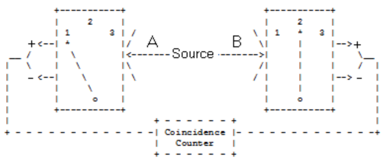
Quantum Correlations Illustrated With Photons
A two-stage atomic cascade emits entangled photons (A and B) in opposite directions with the same circular polarization according to observers in their path. The experiment involves the measurement of photon polarization states in the vertical/horizontal measurement basis, and allows for the rotation of the right-hand detector through an angle \(\theta\), in order to explore the consequences of quantum mechanical entanglement. PA stands for polarization analyzer and could simply be a calcite crystal.
\[\begin{matrix} V & \lhd & \lceil & \; & \rceil & \; & \; & \; & \lceil & \; & \rceil & \rhd & V \\ \; & \; & | & 0 & | & \xleftarrow{A} & \xleftrightarrow{Source} & \xrightarrow{B} & | & \theta & | & \; & \; \\ H & \lhd & \lfloor & \; & \rfloor & \; & \; & \; & \lfloor & \; & \rfloor & \rhd & H \\ \; & \; & PA_{A} & \; & \; & \; & PA_{B} & \; & \; \end{matrix} \nonumber \]
The entangled two-photon polarization state is written in the circular and linear polarization bases,
\[
| \Psi \rangle=\frac{1}{\sqrt{2}}[ |L\rangle_{A} | L \rangle_{B}+| R \rangle_{A} | R \rangle_{B} ]=\frac{1}{\sqrt{2}}[ |V\rangle_{A} | V \rangle_{B}-| H \rangle_{A} | H \rangle_{B} ] \text{using} \quad | L \rangle=\frac{1}{\sqrt{2}}[ |V\rangle+ i | H \rangle ] \quad | R \rangle=\frac{1}{\sqrt{2}}[ |V\rangle- i | H \rangle ]
\nonumber \]
The vertical (eigenvalue +1) and horizontal (eigenvalue -1) polarization states for the photons in the measurement plane are given below. \(\Theta\) is the angle of the measuring PA.
\[
\mathrm{V}(\theta) :=\left( \begin{array}{l}{\cos (\theta)} \\ {\sin (\theta)}\end{array}\right)\quad \mathrm{H}(\theta) :=\left( \begin{array}{l}{-\sin (\theta)} \\ {\cos (\theta)}\end{array}\right) \quad \mathrm{V}(0)=\left( \begin{array}{l}{1} \\ {0}\end{array}\right) \quad \mathrm{H}(0)=\left( \begin{array}{l}{0} \\ {1}\end{array}\right)
\nonumber \]
If photon A has vertical polarization photon B also has vertical polarization, the probability that photon B has vertical polarization when measured at an angle θ giving a composite eigenvalue of +1 is,
\[
\left(\mathrm{V}(\theta)^{\mathrm{T}} \cdot \mathrm{V}(0)\right)^{2} \rightarrow \cos (\theta)^{2}
\nonumber \]
If photon A has vertical polarization photon B also has vertical polarization, the probability that photon B has horizontal polarization when measured at an angle θ giving a composite eigenvalue of -1 is,
\[
\left(\mathrm{H}(\theta)^{\mathrm{T}} \cdot \mathrm{V}(0)\right)^{2} \rightarrow \sin (\theta)^{2}
\nonumber \]
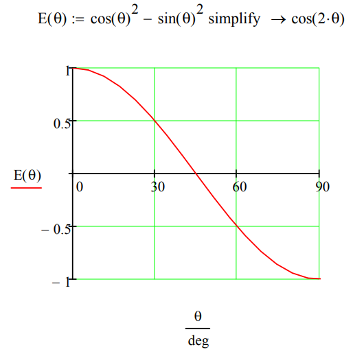
Therefore the overall quantum correlation coefficient or expectation value is:
\[
\mathrm{E}(\theta) :=\left(\mathrm{V}(\theta)^{\mathrm{T}} \cdot \mathrm{V}(0)\right)^{2}-\left(\mathrm{H}(\theta)^{\mathrm{T}} \cdot \mathrm{V}(0)\right)^{2} \text { simplify } \rightarrow \cos (2 \cdot \theta) \quad \mathrm{E}(0 \cdot \mathrm{deg})=1 \quad \mathrm{E}(30 \cdot \mathrm{deg})=0.5 \quad \mathrm{E}(90 \cdot \mathrm{deg})=-1
\nonumber \]
Now it will be shown that a local-realistic, hidden-variable model can be constructed which is in agreement with the quantum calculations for 0 and 90 degrees, but not for 30 degrees (highlighted).
If objects have well-defined properties independent of measurement, the results for \(\theta\) = 0 degrees and \(\theta\) = 90 degrees require that the photons carry the following instruction sets, where the hexagonal vertices refer to \(\theta\) values of 0, 30, 60, 90, 120, and 150 degrees.
There are eight possible instruction sets, six of the type on the left and two of the type on the right. The white circles represent vertical polarization with eigenvalue +1 and the black circles represent horizontal polarization with eigenvalue -1. In any given measurement, according to local realism, both photons (A and B) carry identical instruction sets, in other words the same one of the eight possible sets.
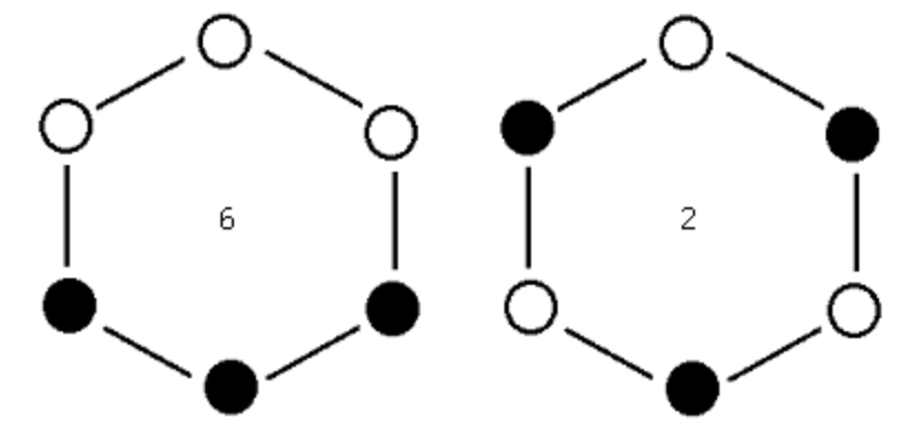
The problem is that while these instruction sets are in agreement with the 0 and 90 degree quantum calculations, with expectation values of +1 and -1 respectively, they can't explain the 30 degree predictions of quantum mechanics. The figure on the left shows that the same result should be obtained 4 times with joint eigenvalue +1, and the opposite result twice with joint eigenvalue of -1. For the figure on the right the opposite polarization is always observed giving a joint eigenvalue of -1. Thus, local realism predicts an expectation value of 0 in disagreement with the quantum result of 0.5.
\[
\frac{6 \cdot(1-1+1+1-1+1)+2 \cdot(-1-1-1-1-1-1)}{8}=0
\nonumber \]
This analysis is based on "Simulating Physics with Computers" by Richard Feynman, published in the International Journal of Theoretical Physics (volume 21, pages 481-485), and Julian Brown's Quest for the Quantum Computer (pages 91-100). Feynman used the experiment outlined above to establish that a local classical computer could not simulate quantum physics.
A local classical computer manipulates bits which are in well-defined states, 0s and 1s, shown above graphically in white and black. However, these classical states are incompatible with the quantum mechanical analysis which is consistent with experimental results. This two-photon experiment demonstrates that simulation of quantum physics requires a computer that can manipulate 0s and 1s, superpositions of 0 and 1, and entangled superpositions of 0s and 1s.
Simulation of quantum physics requires a quantum computer. The following quantum circuit simulates this experiment exactly. The Hadamard and CNOT gates transform the input, |10>, into the required entangled Bell state. R(\(\theta\)) rotates the polarization of photon B clockwise through an angle \(\theta\). Finally measurement yields one of the four possible output states: |00>, |01>, |10> or |11>.
\[\begin{matrix} | 1 \rangle & \rhd & H & \cdot & \cdots & \rhd & \text{Measure 0 or 1} \\ \; & \; & \; & | & \; & \; & \; \\ | 0 \rangle & \rhd & \cdots & \oplus & R(\theta) & \rhd & \text{Measure 0 or 1} \end{matrix} \nonumber \]
The following algebraic analysis of the quantum circuit shows that it yields the correct expectation value for all values of \(\theta\). This analysis requires the truth tables for the matrix operators. Recall from above that |0> = |V> with eigenvalue +1, and |1> = |H> with eigenvalue -1.
\[
H=\left[ \begin{array}{ccc}{0} & {\text { to }} & {\frac{1}{\sqrt{2}} \cdot(0+1)} \\ {1} & {\text { to }} & {\frac{1}{\sqrt{2}} \cdot(0-1)}\end{array}\right] \quad \mathrm{CNOT}=\left( \begin{array}{ccc}{00} & {\mathrm{to}} & {00} \\ {01} & {\mathrm{to}} & {01} \\ {10} & {\mathrm{to}} & {11} \\ {11} & {\mathrm{to}} & {10}\end{array}\right) \quad \begin{matrix} \begin{pmatrix} 1 \\ 0 \end{pmatrix} & \xrightarrow{R(\theta)} & \begin{pmatrix} \cos \theta \\ \sin \theta \end{pmatrix} \\ \begin{pmatrix} 0 \\ 1 \end{pmatrix} & \xrightarrow{R(\theta)} & \begin{pmatrix} - \sin \theta \\ \cos \theta \end{pmatrix} \end{matrix}
\nonumber \]
\[
\begin{array}{c}{|1 \rangle | 0 \rangle=| 10\rangle} \\ {\mathrm{H} \otimes \mathrm{I}}{\frac{1}{\sqrt{2}}[ |0\rangle-| 1 \rangle ] | 0 \rangle=\frac{1}{\sqrt{2}}[ |00\rangle-| 10\rangle} \\ {\text { CNOT }} \begin{array}{c}{\frac{1}{\sqrt{2}}[ |00\rangle-| 11} \\ {\quad \mathrm{I} \otimes \mathrm{R}(\theta)}\end{array}\frac{1}{\sqrt{2}}[ |0\rangle(\cos \theta | 0\rangle+\sin \theta | 1 \rangle )-| 1 \rangle(-\sin \theta | 0\rangle+\cos \theta | 1 \rangle ) ] \\ \Downarrow \\ \frac{1}{\sqrt{2}}[\cos \theta | 00\rangle+\sin \theta | 01 \rangle+\sin \theta | 10 \rangle-\cos \theta | 11 \rangle ] \\ \text{Probabilities} \\ \Downarrow \\ \frac{\cos ^{2} \theta}{2} | 00 \rangle+\frac{\sin ^{2} \theta}{2} | 01 \rangle+\frac{\sin ^{2} \theta}{2} | 10 \rangle+\frac{\cos ^{2} \theta}{2} | 11 \rangle \end{array}
\nonumber \]
|00> = |VV> and |11> = |HH> have a composite eigenvalue of +1. |01> = |VH> and |10> = |HV> have a composite eigenvalue of -1. Therefore,