1.3: Atomic and Molecular Stability

Sometimes practitioners of quantum mechanics misinterpret energy contributions when studying the details of atomic behavior. This can happen when classical concepts are allowed to intrude on the quantum realm where they are not valid.

Another Critique of the Centrifugal Effect in the Hydrogen Atom

On page 174 of Quantum Chemistry & Spectroscopy, 3rd ed. Thomas Engel derives equation 9.5 which is presented in equivalent form in atomic units (\(e = m_{e} = \frac{h}{2 \pi} = 4 \pi \epsilon_{0} = 1\)) here.

\[- \frac{1}{2r^{2}} \frac{d}{dr} (r^{2} \frac{d}{dr} R(r)) + \Bigg[ \frac{L(L+1)}{2r^{2}} - \frac{1}{r} \Bigg] \cdot R(r) = E \cdot R(r) \label{eq1} \]

At the bottom of the page he writes,

Note that the second term (in brackets) on the left‐hand side of Equation 9.5 can be viewed as a effective potential, V_eff(r). It is made up of the centrifugal potential, which varies as +1/r², and the Coulomb potential, which varies as ‐1/r.\[V_{eff} (r) = \frac{L(L+1)}{2r^{2}} - \frac{1}{r} \nonumber \]

Engel notes that because of its positive mathematical sign, the centrifugal potential is repulsive, and goes on to say,

The net result of this repulsive centrifugal potential is to force the electrons in orbitals with L > 0 ( p, d, and f electrons) on average farther from the nucleus than s electrons for which L = 0.

This statement is contradicted by the radial distribution functions shown in Figure 9.10 on page 187, which clearly show the opposite effect. As L increases the electron is on average closer to the nucleus. It is further refuted by calculations of the average value of the electron position from the nucleus as a function of the n and L quantum numbers. For a given n the larger L is the closer on average the electron is to the nucleus. In other words, these calculations support the graphical representation in Figure 9.10.

\[r(n,L) \colon = \frac{3n^{2} - L(L+1)}{2} \quad \begin{pmatrix} L & 0 & 1 & 2 & 3 \\ n=1 & 1.5 & ' & ' & ' \\ n=2 & 6 & 5 & ' & ' \\ n=3 & 13.5 & 12.5 & 10.5 & ' \\ n=4 & 24 & 23 & 21 & 18 \end{pmatrix} \nonumber \]

On page 180 in Example Problem 9.2, Engel introduces the virial theorem. For systems with a Coulombic potential energy, such as the hydrogen atom, it is

\[\langle V \rangle = 2 \langle E \rangle = ‐2 \langle T \rangle. \nonumber \]

We will work with the version

\[\dfrac{ \langle E \rangle}{\langle V \rangle} = 0.5. \nonumber \]

The values of the energy, the so called centrifugal potential energy and the Coulombic potential energy are as shown below as a function of the appropriate quantum numbers.

\[E(n) \colon = \frac{-1}{2n^{2}} \qquad V_{centrifugal} (n,L) \colon = \frac{L(L+1)}{2n^{3} (L+ \frac{1}{2})} \qquad V_{coulomb} (n) \colon = - \frac{1}{n^{2}} \nonumber \]

The calculations below show that the virial theorem is violated for any state for which L > 0.

\[1s \quad n \colon = 1 \quad L \colon = 0 \quad \frac{E(n)}{V_{centrifugal} (n,L) + V_{coulomb} (n)} = 0.5 \nonumber \]

\[2s \quad n \colon = 2 \quad L \colon = 0 \quad \frac{E(n)}{V_{centrifugal} (n,L) + V_{coulomb} (n)} = 0.5 \nonumber \]

\[2p \quad n \colon = 2 \quad L \colon = 1 \quad \frac{E(n)}{V_{centrifugal} (n,L) + V_{coulomb} (n)} = 0.75 \nonumber \]

\[3s \quad n \colon = 3 \quad L \colon = 0 \quad \frac{E(n)}{V_{centrifugal} (n,L) + V_{coulomb} (n)} = 0.5 \nonumber \]

\[3p \quad n \colon = 3 \quad L \colon = 1 \quad \frac{E(n)}{V_{centrifugal} (n,L) + V_{coulomb} (n)} = 0.643 \nonumber \]

\[3d \quad n \colon = 3 \quad L \colon = 2 \quad \frac{E(n)}{V_{centrifugal} (n,L) + V_{coulomb} (n)} = 0.833 \nonumber \]

These calculations are now repeated eliminating the centrifugal term, showing that the virial theorem is satisfied and supporting the claim that the ʺcentrifugal potentialʺ is actually a kinetic energy term.

\[1s \quad n \colon = 1 \quad L \colon = 0 \quad \frac{E(n)}{V_{coulomb} (n)} = 0.5 \nonumber \]

\[2s \quad n \colon = 2 \quad L \colon = 0 \quad \frac{E(n)}{V_{coulomb} (n)} = 0.5 \nonumber \]

\[2p \quad n \colon = 2 \quad L \colon = 1 \quad \frac{E(n)}{V_{coulomb} (n)} = 0.5 \nonumber \]

\[3s \quad n \colon = 3 \quad L \colon = 0 \quad \frac{E(n)}{V_{coulomb} (n)} = 0.5 \nonumber \]

\[3p \quad n \colon = 3 \quad L \colon = 1 \quad \frac{E(n)}{V_{coulomb} (n)} = 0.5 \nonumber \]

\[3d \quad n \colon = 3 \quad L \colon = 2 \quad \frac{E(n)}{V_{coulomb} (n)} = 0.5 \nonumber \]

We finish by rewriting Equation \ref{eq1} with brackets showing that the first two terms are quantum kinetic energy and that the Coulombic term is the only potential energy term.

\[\Bigg[ - \frac{1}{2r^{2}} \frac{d}{dr} (r^{2} \frac{d}{dr} R(r)) + \frac{L(L+1)}{2r^{2}} \cdot R(r) \Bigg] - \frac{1}{r} \cdot R(r) = E \cdot R(r) \nonumber \]

In summary, the ʺcentrifugal potentialʺ and the concept of ʺeffective potential energyʺ are good examples of the danger in thinking classically about a quantum mechanical system. Furthermore, itʹs bad pedagogy to create fictitious forces and to mislabel energy contributions in a misguided effort to provide conceptual simplicity.

---

Further evidence that confinement energy is not kinetic energy is seen in the following analysis of the effect of lepton mass in the hydrogen atom. In what follows the electron is replaced by the muon and the tauon in the hydrogen atom. Positronium, in which the proton is replaced by the positron, is also examined. These analyses also provide a graphical illustration of the uncertainty principle.

Exploring the Role of Lepton Mass in the Hydrogen Atom

Under normal circumstances the the hydrogen atom consists of a proton and an electron. However, electrons are leptons and there are two other leptons which could temporarily replace the electron in the hydrogen atom. The other leptons are the muon and tauon, and their fundamental properties, along with those of the electron, are given in the following table.

\[\begin{pmatrix} \text{Property} & e & \mu & \tau \\ \frac{Mass}{m_{e}} & 1 & 206.8 & 3491 \\ \frac{Effective\; Mass}{m_{e}} & 1 & 185.86 & 1203 \\ \frac{Life\; Time}{s} & Stable & 2.2 \times 10^{-6} & 3.0 \times 10^{-13} \end{pmatrix} \nonumber \]

The purpose of this exercise is to demonstrate the importance of mass in atomic systems, and therefore also kinetic energy. Substitution of the deBroglie relation (\(\lambda = \frac{h}{m \nu}\)) into the classical expression for kinetic energy yields a quantum mechanical expression for kinetic energy. It is of utmost importance that in quantum mechanics, kinetic energy is inversely proportional to mass.

\[T = \frac{1}{2} mv^{2} = \frac{h^{2}}{2m \lambda^{2}} \nonumber \]

A more general and versatile quantum mechanical expression for kinetic energy is the differential operator shown below, where again mass appears in the denominator. An Approach to Quantum Mechanics outlines the origin of kinetic energy operator.

Atomic units (\(e = m_{e} = \frac{h}{2 \pi} = 4 \pi \epsilon_{0} = 1\)) will be used in the calculations that follow. Please note that \(\mu\) in the equations below is the effective mass and not a symbol for the muon.

Kinetic energy operator:$$T= - \frac{1}{2 \mu r} \frac{d^{2}}{dr^{2}} ( \cdot \Box)$$

Potential energy operator:$$V = - \frac{1}{r} \cdot \Box$$

Variational trial wave function with variational parameter \(\beta\):

\[\Psi (r, \beta) \colon = \left(\dfrac{\beta^{3}}{\pi}\right)^{1/2} \cdot \exp (- \beta \cdot r) \nonumber \]

Evaluation of the variational energy integral:

\[E(\beta , \mu) \colon = \int_{0}^{\infty} \Psi (r, \beta) \Bigg[ - \frac{1}{2 \mu r} \frac{d^{2}}{dr^{2}} (r \cdot \Psi (r, \beta) \Bigg] 4 \pi r^{2} \; dr \ldots \bigg|_{\text{simplify}}^{\text{assume,}\; \beta > 0} \rightarrow \frac{\beta^{2}}{2 \mu} - \beta + \int_{0}^{\infty} \Psi (r, \beta) \cdot - \frac{1}{r} \cdot \Psi (r, \beta) \cdot 4 \pi r^{2}\; dr \nonumber \]

Minimize the energy with respect to the variational parameter \(\beta\).

\[\frac{d}{d \beta} E( \beta, \mu) = 0\; \text{solve,}\; \beta \rightarrow \mu \nonumber \]

Express energy in terms of reduced mass:

\[E( \beta , \mu)\; \text{substitute,} \; \beta = \mu \rightarrow - \frac{\mu}{2} \nonumber \]

Using the virial theorem the kinetic and potential energy contributions are:

\[T = \frac{\mu}{2} \qquad V = - \mu \nonumber \]

Express the trial wave function in terms of reduced mass.

\[\Psi (r, \beta)\; \text{substitute,}\; \beta = \mu \rightarrow \frac{e^{- \mu r} \sqrt{\mu^{3}}}{\sqrt{\pi}} \nonumber \]

Demonstrate the effect of mass on the radial distribution function with plots of mass equal to 0.5, 1 and 2.

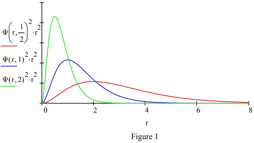
Calculate the expectation value for position to show that it is consistent with the graphical representation above. The more massive the lepton the closer it is on average to the proton.

\[\int_{0}^{\infty} \Psi (r, \mu) \cdot r \cdot \Psi (r, \mu) \cdot 4 \pi r^{2}\; dr\; \text{assume,}\; \mu > 0 \rightarrow \frac{3}{2 \mu} \nonumber \]

Summarize the calculated values for the physical properties of H_e, H_\(\mu\) and H_\(\tau\).

\[\begin{pmatrix} \text{Species} & \frac{E}{E_{h}} & \frac{T}{E_{h}} & \frac{V}{E_{h}} & \frac{r_{avg}}{a_{0}} \\ H_{e} & \frac{-1}{2} & \frac{1}{2} & -1 & \frac{3}{2} \\ H_{\mu} & -92.93 & 92.93 & -185.86 & 8.07 \times 10^{-3} \\ H_{\tau} & -601.5 & 601.5 & -1203 & 1.25 \times 10^{-3} \end{pmatrix} \nonumber \]

Now imagine that you have a regular hydrogen atom in its ground state and the electron is suddenly by some mechanism replaced by a muon. Nothing has changed from an electrostatic perspective, but the change in energy and average distance of the lepton from the proton are very large. The ground state energy and the average distance from the nucleus decrease by a factor of 185.6, the ratio of the effective masses of the electron and the muon.

This mass effect provides a challenge for those who think all atomic physical phenomena can be explained in terms of electrostatic potential energy effects. Of course, there is an even bigger problem for the potential energy aficionados, and that is the fundamental issue of atomic and molecular stability. Quantum mechanical kinetic energy effects are required to explain the stability of matter.

A Fourier transform of the coordinate wave function yields the corresponding momentum distribution and the opportunity to create a visualization of the uncertainty principle.

\[\Phi (p, \mu) \colon = \frac{1}{4 \sqrt{\pi^{3}}} \int_{0}^{\infty} \exp(-ipr) \cdot \Psi (r, \mu) \cdot 4 \pi r^{2} \; dr \bigg|_{\text{simplify}}^{\text{assume,}\; \mu > 0} \rightarrow \frac{2 \mu^{3/2}}{\pi (\mu + p \cdot i)^{3}} \nonumber \]

Figure 2 shows that the most massive particle has the most delocalized momentum distribution. This is consistent with the uncertainty principle which states less spatial uncertainty is accompanied by greater uncertainty in the momentum distribution.

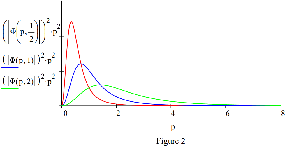
Replacing the proton with a positron, the electron's anti-particle, creates another exotic atom, positronium (Ps). In its singlet ground state electron-positron annihilation occurs in 125 ps creating two \(\gamma\) rays. Positronium's (\(\mu\) = 1/2) spatial and momentum distributions are shown in Figures 1 and 2. A revised table including positronium is provided below.

\[\begin{pmatrix} \text{Species} & \frac{E}{E_{h}} & \frac{T}{E_{h}} & \frac{V}{E_{h}} & \frac{r_{avg}}{a_{0}} \\ H_{e} & - \frac{1}{2} & \frac{1}{2} & -1 & \frac{3}{2} \\ H_{\mu} & -92.93 & 92.93 & -185.86 & 8.07 \times 10^{-3} \\ H_{\tau} & -601.5 & 601.5 & -1203 & 1.25 \times 10^{-3} \\ Ps & - \frac{1}{4} & \frac{1}{4} & - \frac{1}{2} & 3 \end{pmatrix} \nonumber \]

---

Many in the chemical education community teach chemical bonding as simply an electrostatic phenomenon. I and many others have argued against this incorrect, simplistic view on many occasions. In an effort to get a better understanding let’s look at an overview of the nature of the chemical bond written by Frank E. Harris many years ago.

The Chemical Bond and Quantum Mechanics*

The behavior of electrons in molecules and atoms is described by quantum mechanics; classical (Newtonian) mechanics cannot be used because the de Broglie wavelengths (\(\lambda= \frac{h}{m \nu}\)) of the electrons are comparable with molecular (and atomic) dimensions. The relevant quantum-mechanical ideas are as follows:

• Electrons are characterized by their entire distributions (called wave functions or orbitals) rather than by instantaneous positions and velocities: an electron may be considered always to be (with appropriate probability) at all points of its distribution (which does not vary with time).
• The kinetic energy of an electron decreases as the volume occupied by the bulk of its distribution increases, so delocalization lowers its kinetic energy.$$KE= \frac{p^{2}}{2m} = \frac{h^{2}}{2m \lambda^{2}} \approx \frac{A}{D^{2}} \approx \frac{A}{V^{2/3}}$$
• The potential energy of interaction between an electron and other charges is as calculated by classical physics, using the appropriate distribution (wave function) for the electron: an electron distribution is therefore attracted by nuclei and its potential energy decreases as the average electron-nuclear distance decreases.$$PE \approx - \frac{B}{D} \approx - \frac{B}{V^{1/3}}$$
• A minimum-energy electron distribution represents the best compromise between concentration near the nuclei (to reduce potential energy) and delocalization (to reduce kinetic energy).$$E = KE + PE \approx \frac{A}{V^{2/3}} - \frac{B}{V^{1/3}}$$

A bond will form between two atoms when the electron distribution of the combined atoms (molecular orbital) yields a significantly lower energy than the separate-atom distributions (atomic orbitals). An example is a covalent bond, in which two electrons, one originally on each atom, change their distributions so that each extends over both atoms.

---

* Taken from "Molecules" in The Encyclopedia of Physics by Frank E. Harris (with some additions and modifications by Frank Rioux)

We go deeper with the following treatment of the covalent bond in the hydrogen molecule ion using the virial theorem (John C. Slater) and ab initio quantum mechanics (Klaus Ruedenberg). In my opinion, Slater and Ruedenberg are the true pioneers in understanding the covalent chemical bond. Many books have been written about the chemical bond, but few are as insightful as the papers published by Slater and Ruedenberg.

Two Analyses of the Covalent Bond Using the Virial Theorem

Atomic and molecular stability and spectroscopy, and the nature of the chemical bond cannot be explained using classical physics: quantum mechanical principles are required. Bohr was a pioneer in an effort to apply an early version of quantum theory to these important issues with his models of the hydrogen atom and hydrogen molecule. Of course, Bohr's approach became "old" quantum mechanics and was abandoned in the 1920s with the creation of a "new" quantum mechanics by Heisenberg and Schrödinger and their collaborators. This tutorial deals exclusively with the chemical bond and summarizes Slater's contribution to our current understanding of the energetics of its formation using the virial theorem. Since the acceptance of the "new" quantum mechanics many others have contributed to the interpretation of chemical bond formation, but like Bohr, Slater was an insightful pioneer.

In a seminal paper, J.Chem. Phys. 1933, 1, 687-691, John C. Slater used the virial theorem to analyze chemical bond formation and was the first (in my opinion) to recognize the importance of kinetic energy in covalent bond formation. Regarding the universally valid virial theorem he wrote,

...this theorem gives a means of finding kinetic and potential energy separately for all configurations of the nuclei, as soon as the total energy is known, from experiment or theory.

The purpose of this tutorial is to demonstrate the validity of this assertion. The experimental method employs a Morse function for the energy of the hydrogen molecule ion parametrized using spectroscopic data. The theoretical approach is based on an ab initio LCAO-MO calculation of the energy based on a molecular orbital consisting a superposition of scaled hydrogen atomic orbitals.

Experimental Method

The kinetic energy, potential energy and total energy of the hydrogen molecule ion are calculated as a function of R using the virial theorem and a Morse function for the total energy based on experimental parameters.

Total energy:	$$E(R) = T(R) + V(R) \tag{1}$$
Virial theorem:	$$2 \cdot T(R) + V(R) = - R \frac{d}{dR} E(R) \tag{2}$$
Morse parameters:	$$D_{e} : = 0.103 \cdot E_{h} \qquad R_{e} : = 2.003 \cdot a_{0} \qquad \beta : = 0.708 a_{0}^{-1}$$

These parameters are from Levine, I. N. Quantum Chemistry, 6th ed., p. 400.

Morse Function:

\[E(R) : = D_{e} (1- \exp [ - \beta (R - R_{e})])^{2} - D_{e} \tag{3}$$

Using equation (1) to eliminate V(R) in equation (2) yields an equation for kinetic energy as a function of the internuclear separation. Using equation (1) to eliminate T(R) in equation (2) yields an equation for potential energy as a function of the internuclear separation.

\[T(R) : = -E(R) - R \frac{d}{dR} E(R) \tag{4} \]

\[V(R) : = 2 E(R) + R \frac{d}{dR} E(R) \tag{5} \]

These important equations determine the mean kinetic and potential energies as functions of R, one might almost say experimentally, directly from the curves of E as a function of R which can be found from band spectra. The theory is so simple and direct that one can accept the results without question....

\[R : = 0.6 a_{0}, 0.65 a_{0} \ldots 8a_{0} \nonumber \]

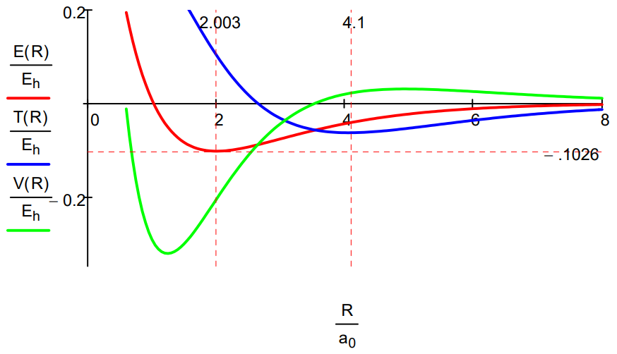
While the Morse calculation has an empirical flavor to it, its results are interpreted in terms of rudimentary quantum theory concepts. This energy profile shows that as the protons approach, the potential energy rises because molecular orbital formation (constructive interference) draws electron density away from the nuclei into the internuclear region. The kinetic energy decreases because molecular orbital formation brings about electron delocalization.

At about 4.1a₀ this trend reverses as atomic orbital contraction begins. The kinetic energy rises because the volume occupied by the electron decreases and the potential energy decreases for the same reason: a smaller electronic volume brings the electron closer to the nuclei on average. Only at R ~ 1a₀ does nuclear repulsion cause the total potential energy to increase and contribute to the repulsion energy of the molecule. In other words, the kinetic energy increase is the immediate cause of the energy minimum or ground state.

Theoretical Method

The following LCAO-MO calculation uses a superposition of scaled 1s atomic orbitals and yields the following result for the energy of the hydrogen molecule ion as a function of the internuclear distance and the orbital scale factor.

\[1s_{a} = \sqrt{\frac{\alpha^{3}}{\pi}} \exp (- \alpha r_{a}) \nonumber \]

\[1s_{b} = \sqrt{\frac{\alpha^{3}}{\pi}} \exp (- \alpha r_{b}) \nonumber \]

\[S_{ab} = \int 1s_{a} \cdot 1s_{b} d \tau \nonumber \]

\[\Psi_{mo} = \frac{1s_{a} + 1s_{b}}{\sqrt{2+2S_{ab}}} \nonumber \]

\[E(\alpha , R) : = \frac{- \alpha^{2}}{2} + \frac{[\alpha^{2} - \alpha - \frac{1}{R} + \frac{1 + \alpha R}{R} \exp (-2 \alpha R) + \alpha (\alpha - 2) \cdot (1 + \alpha R) \exp (- \alpha R)]}{[1+ \exp(- \alpha R) \cdot (1 + \alpha R + \frac{\alpha^{2} R^{2}}{3})]} + \frac{1}{R} \nonumber \]

\(\alpha\) := 1

Energy := 2

\[\text{Given}\; Energy = E (\alpha ,R) \quad \frac{d}{d \alpha} E( \alpha ,R) = 0 \quad Energy(R) := Find(\alpha, Energy) \nonumber \]

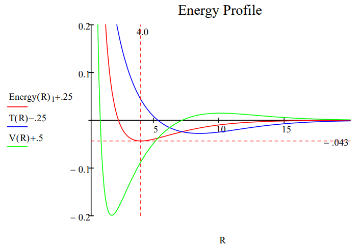
As noted above, using \(E=T+V\) with the virial theorem \(2T+V=-R \frac{d}{dR} E\) leads to the following expressions for T and V.

\[T(R) := - Energy(R)_{1} - R \frac{d}{dR} Energy (R)_{1} \qquad V(R) := 2 \cdot Energy(R)_{1} + R \frac{d}{dR} Energy(R)_{1} \qquad R := 0.2, 0.25 \ldots 10 \nonumber \]

It is clear that both methods lead to very similar energy profiles. The only significant difference is that the Morse calculation leads to a lower energy minimum, -0.1026 E_h versus -0.0865 E_h for the molecular orbital calculation. Therefore, the interpretation provided for the Morse energy profile is valid for the LCAO-MO profile.

Conversion factors: \(a_{0} = 5.29177 \cdot 10^{-11}\; m \qquad E_{h} = 4.359748 \cdot 10^{-18}\; joule\)

---

The following link provides graphical displays of the electron density in the hydrogen molecule ion.

The following calculation shows that the lepton mass effect in molecules is the same as it is atoms. This mass effect provides a challenge for those who think atomic and molecular stability can be explained solely in terms of electrostatic potential energy effects. The mass effect is important because quantum mechanical kinetic energy (confinement energy) is inversely proportional to mass, but classical kinetic energy is directly proportional to mass.

A Molecular Orbital Calculation for H₂⁺

An ab initio molecular orbital calculation yields the following result for the energy of the hydrogen molecule ion as a function of the internuclear separation, lepton mass (highlighted below) and the orbital decay constant.

\[
1 \mathrm{s}_{\mathrm{a}}=\sqrt{\frac{\alpha^{3}}{\pi}} \cdot \exp \left(-\alpha \cdot r_{\mathrm{a}}\right) \qquad 1 s_{b}=\sqrt{\frac{\alpha^{3}}{\pi}} \cdot \exp \left(-\alpha \cdot r_{b}\right) \qquad \mathrm{S}_{\mathrm{ab}}=\int \quad \mathrm{1s}_{\mathrm{a}} \cdot 1 \mathrm{s}_{\mathrm{b}} \mathrm{d} \tau \qquad \Psi_{\mathrm{mo}}=\frac{1 \mathrm{s}_{\mathrm{a}}+\mathrm{ls}_{\mathrm{b}}}{\sqrt{2+2 \cdot \mathrm{s}_{\mathrm{ab}}}}
\nonumber \]

\[
m : = 0.5 \quad \mathrm{E}(\alpha, \mathrm{R}) :=\frac{-\alpha^{2}}{2 \cdot \mathrm{m}}+\frac{\frac{\alpha^{2}}{\mathrm{m}}-\alpha-\frac{1}{\mathrm{R}}+\frac{1}{\mathrm{R}} \cdot(1+\alpha \cdot \mathrm{R}) \cdot \exp (-2 \cdot \alpha \cdot R)+\alpha \cdot\left(\frac{\alpha}{m}-2\right) \cdot(1+\alpha \cdot R) \cdot \exp (-\alpha \cdot R)}{1+\exp (-\alpha \cdot R) \cdot\left(1+\alpha \cdot R+\frac{\alpha^{2} \cdot R^{2}}{3}\right)}+\frac{1}{R}
\nonumber \]

\[
\alpha : = 1 \quad \text{Energy} : = -2 \qquad \text{Given} \quad \text{Energy} = E(\alpha, R) \quad \frac{d}{d \alpha} E( \alpha ,R) = 0 \quad \text{Energy(R)} : = \text{Find} (\alpha , \text{Energy}) \nonumber \]

Using \(E = T + V\) in the virial theorem \(2 T + V = -R \cdot \frac{d}{dR} E\) yields expressions for T and V.

\[R : = 0.2, 0.3 \ldots 20 \quad \mathrm{T}(\mathrm{R}) :=-\text { Energy }(\mathrm{R})_{1}-\mathrm{R} \cdot \frac{\mathrm{d}}{\mathrm{dR}} \text { Energy }(\mathrm{R})_{1} \quad \mathrm{V}(\mathrm{R}) :=2 \cdot \text { Energy }(\mathrm{R})_{1}+\mathrm{R} \cdot \frac{\mathrm{d}}{\mathrm{dR}} \text { Energy( R } )_{1} \nonumber \]

Note that halving the lepton mass reduces the ground state energy by half and doubles the bond length. The same mass effect was found earlier for the hydrogen atom.

---

Some might feel uncomfortable relying on a one-electron molecule to gain an understanding of the chemical bond. After all don’t chemical bonds consist of electron pairs? So we move to the hydrogen molecule for a quantum analysis of the more traditional two-electron bond. The only new contribution to the total energy is electron-electron potential energy, and the significance of confinement energy in understanding molecular stability survives.